
Jump to
- Abstract
- 1. Introduction
- 2. Building an integrated CGE model with many households and separating the household sector
- 3. Solving the BMS model in a CGE framework iteratively
- 4. Revising the BMS model to introduce more flexible functional forms
- 5. Some concluding remarks
- Footnotes
- Appendix
- References
- Article and author information
1. Introduction
Computable general equilibrium (CGE) models are very useful for analysing the impacts of policy changes on the economy as a whole. However, as CGE models are typically built on the basis of input-output tables, many sub-sectoral details are often omitted due to aggregation. For microeconomic analysis at the sub-sectoral or sub-regional level, the most useful tool is the partial equilibrium (PE) model. Due to the different characteristics of individual sectors or regions analysed, the types of PE models vary widely, ranging from behavioural microsimulation (BMS) models with large samples of households to detailed industry-specific models with individual firms and their unique cost structures or technologies1.
Researchers have tried to bring the two types of models together to overcome their respective limitations, by integrating micro data and behaviour into a CGE framework. There are two major approaches. One is the so-called top-down (TD) approach, in which the simulation results of a CGE model are transmitted to a PE model, where the corresponding variables are exogenous, to gain a sense of distributional effects. For example, a microsimulation (MS) model might be used to calculate the effects of changes in wages and prices on individual households’ budgets. In this approach any household responses in terms of consumer demands and factor supplies are not fed back to the CGE model. Despite this limitation, this approach remains popular among researchers, mainly due to its simplicity and ease of implementation2.
The other approach is more sophisticated and known as the top down-bottom up (TD-BU) approach. In addition to the top-down effects from a CGE model, this approach also takes into account the “bottom-up” responses to the initial CGE changes of individual households from a behavioural microsimulation (BMS) model. This feedback effect enables the CGE model to account for behavioural responses from the BMS model. Typically, the CGE model is provided with quantity changes from the BMS model, while the BMS model is provided with price changes from the CGE models. This approach requires two models to perform iterative simulations until their solutions converge. Bourguignon and Savard (2008) refer to this process of iterating between prices and quantities as a fixed point algorithm3.
Savard (2003) links a CGE model and a BMS model to simulate the distributional impacts of a tariff reduction on a large number of households in the Philippines (see also, Bourguignon & Savard, 2008). A sample of similar studies includes: Fredriksen, Heide, Holmoy, and Solli (2007) who combine a dynamic microsimulation model of government pension expenditures and a large CGE-model of the Norwegian economy to estimate the extent to which two reforms of the public pension system might improve fiscal sustainability and stimulate employment. Aaberge Colombino, Holmøy, Strøm, and Wennemo (2007) link a micro model of household labour supply with a CGE model of the Norwegian economy to analyse the impacts of population ageing. Both studies solve the models iteratively, with changes in labour supply determined by the micro model and used by the CGE, which determine changes in wage rates, cash transfers and capital income.
Savard notes, however, an important limitation in this approach, “nothing guarantee[s] a converging solution to be found; therefore it must be validated and numerically checked for the introduction of each new hypothesis” (Savard, 2003, p. 8)4. In a recent survey of microsimulation models, Cockburn, Savard, and Tiberti (2014, p. 8) also conclude that the ‘main shortcoming of this technique is that convergence is not guaranteed and must be verified for each simulation’.
The lack of convergence typically originates from the two linked models having different behavioural assumptions or using inconsistent databases. Typically, a BMS model includes consumer demands for each household, whereas, in most CGE models, especially those used in TD-BU, consumer demand is modelled for a single representative household. These two demand systems can be difficult to reconcile5. If the two databases are also not fully consistent, a convergent solution can be even more difficult to reach6. More importantly, the data inconsistency could distort the simulation results. As Colombo (2010, p. 90) notes, “data inconsistencies between the micro and the macro datasets can also affect results seriously […] one is left unable to distinguish which is the part of the resulting change that is due to feedback effects and which is the part due to data inconsistencies.”
The issue of data inconsistency can only be resolved by adjusting the datasets. In fact, data reconciliation paves the way for developing a more integrated approach, in which a PE sub-model is integrated fully into a CGE model. Although the idea of integrated models is not a new one, only limited attempts have been made to build fully integrated models to date7. Some practical difficulties prevent this approach from being adopted widely. One of the difficulties is the problem of dimensionality: the micro dataset can be too large, making the integrated model difficult to solve. A more serious problem is the difficulty of introducing complex functional forms or discrete rules and conditions, commonly used in PE models, into a CGE framework, particularly when it is written in percentage change form. As CGE models are typically built with smooth, “well-behaved” functions to make them tractable, introducing the kind of complexities that are found in PE models could make a CGE model unsolvable8. This is why, despite the integrated approach being compelling in principle, in practice, some integrated models have been decomposed into two separate models and solved iteratively.
For instance, Rutherford, Tarr, and Shepotylo (2004) integrated over 30,000 household types in a CGE model to analyse the distributional impacts of Russia’s accession to the World Trade Organisation (WTO). As the integrated model was too large to be solved efficiently, a disaggregated household module was separated from the CGE model and the two models were solved iteratively. However, as the aggregate household in the CGE model has its own demand function, different from that of the disaggregated households, an algorithm was required so that, in each iteration, the demand parameters in the CGE model could be recalibrated to emulate the solution obtained from the household model, effectively neutralising the original aggregate household behaviour in the CGE model.
Arntz, Boeters, and Gürtzgen (2005) integrate a discrete choice labour supply function into a CGE model with 26 household groups. Arntz, Boeters, Gürtzgen, and Schubert (2006) extend this model to include 3,000 household types to analyse German welfare reform proposals designed to encourage labour force participation. This model proved too big to solve as a single model so the authors separated the two models and solve the system iteratively. With only one variable (aggregate labour supply) to link, the authors found that two models converged quickly.
There seems to be a dilemma in trying to bring detailed household activities into CGE models. On the one hand, the integrated model is compelling, but it cannot fully incorporate complex PE model behaviours because doing so makes the integrated model intractable. On the other hand, the iterative approach does not guarantee a convergent solution. Obtaining a valid solution depends largely on trial-and-error or continuous adjustments to one model to match the other - a long procedure with an uncertain outcome. The challenge is, therefore, to find a modelling approach, which (a) is flexible enough to allow complex functional forms or conditions to be included in a GE framework; (b) is powerful enough to solve models with large datasets quickly; (c) always produces a converging and GE solution.
In fact, if a PE model can be solved as part of an integrated CGE model, it should be possible for the same PE model to be solved outside the CGE model, using an iterative method to produce the same solution. The success of such a method relies on two conditions: (a) the databases of the two models must be fully consistent with each other; and (b) the two models must be structurally dependent on each other without overlapping behavioural functions. In a CGE-BMS context, the CGE model should have no household behaviour, and the BMS model should have no price formation mechanism. The missing components of one model are exclusively determined by reference to the other. In other words, the two models are not standalone: they are “separate, but integrated”.
The first condition ensures that the solution is not affected by any database discrepancies while the second condition ensures that the separate PE model is still a part of the overall CGE model. Under these conditions, if the correct linking variables are used, iterative simulations should produce a convergent solution and no additional calibrating algorithms, such as those used in Rutherford et al. (2004) are needed.
In this paper, an integrated model provides a starting point for building such structurally linked models. Take an integrated model with multiple households as an example. The household module can be solved as an integrated component of the CGE model using conventional solution methods. Alternatively, the CGE model can be partitioned so that the household module is solved as a separate sub-model conditional on the rest of the CGE model. As the households in the sub-model are price takers, they respond to a given set of price changes by adjusting their demands for goods and supplies of factors. These quantity responses are aggregated to determine the behaviour of the aggregate household in the CGE model to solve for a new set of equilibrium prices to be used in the next iteration. As the two separate models complement each other structurally, these iterations emulate the interactions that the household module would have with the rest of the CGE model if it were solved as a fully integrated model. As a result, a convergent solution should be expected and should always be identical to that from the integrated model9.
More importantly, as the sub-model is outside the CGE model’s equation system and solved separately, it becomes free from the constraints that some conventional solution methods impose on the CGE model. As a result, the sub-model can be modified to incorporate more sophisticated functional forms or policy rules that would jeopardise the tractability of the model.
In a household module, more flexible behavioural assumptions or discrete rules and complex conditions for tax and transfer payments at the individual household or person level can be readily implemented. Moreover, the sub-model can also be written in any form, linear or nonlinear, not necessarily in the same form as the CGE model. So long as these modifications do not alter the initial data consistency with the main model, a convergent and undistorted solution remains guaranteed.
This paper will use an integrated CGE model with a large sample of Australian households as an example to illustrate how the approach is implemented. The remainder of this paper is organised as follows.
In Section 1, a simple-structured CGE model of the Australian economy and an Australian household survey dataset are used to build an integrated CGE model in which the aggregate consumption function of a single representative household is replaced by the individual consumption functions of a large number of household types10. In this model, for simplicity, each household is assumed to display Cobb-Douglas preferences, which are parameterised with its own unique consumption pattern11. This integrated CGE model is first solved using conventional solution techniques. Once the existence of a GE solution is confirmed, the household module is then separated from the integrated model to be used as a separate household sub-model, referred to as a BMS12 model. The remainder of the integrated model is reduced to a conventional one.
However, the representative household in this model becomes an accounting unit with no behaviour13.
Section 2 illustrates how to solve a BMS model with a linked CGE model iteratively. Two cases are discussed. In the first case, the household BMS model, developed in the first section, is solved iteratively with the CGE model to demonstrate that a convergent solution can be found and, more importantly, that the solution is identical to that from the integrated model, a true GE solution. As the two solutions converge quickly without any complication, this case is regarded as well-behaved. A second and more complex example is also presented to show how the same iterative approach can be used to find a convergent GE solution when a model is not well behaved. The second example may represent a more general case, in which a slack variable is required for realigning the household budgets between the two linked models in the iteration process.
Section 3 shows that, once the iterative solution is verified, the same database can be used to build a different BMS model, with more complex behavioural assumptions, and discrete rules and conditions for income tax and transfer payments14. The paper modifies the simple BMS model to introduce a more realistic income tax schedule and a truncated labour supply function to show that it can still be solved iteratively with the CGE model to produce a convergent and GE solution.
The paper concludes with some comments on the possible applications of the ideas behind the iterative approach to partitioning of other parts of a CGE model. The paper focuses on how and under what conditions convergence is achieved, instead of the actual simulation results. For GEMPACK15 users, a simple and effective way of linking and iteratively solving separate models is provided in Appendix A.
2. Building an integrated CGE model with many households and separating the household sector
This section outlines a procedure for creating a detailed household model that accounts for market interactions. The process starts from building a CGE model that integrates a detailed household module. It shows how the household module is taken out of the integrated model to form a separate BMS model and how the BMS model is linked with the rest of the CGE model. Although it is not necessary to follow this approach, an important advantage of building a BMS model from an integrated model is that it ensures the BMS database is fully consistent with the CGE database.
The integrated model database is drawn from two sources: a 104-industry input-output table (Australian Bureau of Statistics, 2015) and household survey data for 9,774 sample households and more than 18,000 persons (Australian Bureau of Statistics, 2012). The method used to reconcile the two datasets is detailed in Appendix B. The model consists of 40 equations, which are essential for the model’s general equilibrium solution. A full list of the core equations is provided in Appendix C.16
The household module is included in Sections 5 and 6 of the integrated model, provided in Appendix C. It has 11 equations (Equations 30–40) and, therefore, it is easy to take it out of the integrated model’s system and use it as a separate BMS model. This sub-model consists of two sections: one defines various sources of household income and demands for goods and services; the other calculates a set of aggregate variables that are used in linking with their counterparts in the CGE model. In this implementation, the CGE assumptions about fixed factor supplies, income tax rates and real transfer payments remain unchanged so that the solutions from the integrated and the iterative models are comparable. These assumptions will be relaxed in Section 3, when the BMS model is modified to introduce household labour supply behaviour and more complex income tax rules.
Initially, the individual household saving rates,
With the household module taken out, the integrated model is reduced to a conventional CGE model with only one representative household. However, it has a fundamental difference from a conventional model: it becomes ‘incomplete’ because it has no household behaviour. The household behaviour has been ‘decomposed out’. The household sector is an accounting unit: the behaviour of the aggregate household is simply the aggregation of individual household behaviours as taken from the BMS model. The CGE model uses some aggregate variables to link with the BMS model: total factor supplies
The household model, formed with the 11 equations from the integrated model, takes changes in all prices and in the average saving rate from the CGE model – the factor price variables
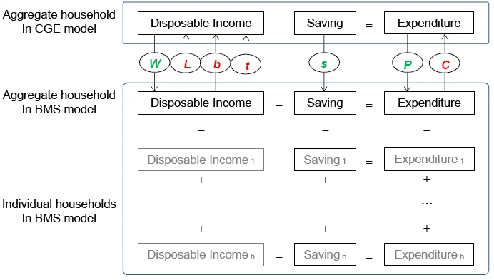
In the two initial databases, the aggregate household budgets are identical and balanced: disposable income, net of savings, equals expenditure. Disposable income is equal to factor income (WL) plus transfer payments (b), net of income tax (t). When the household module is separated from the CGE model, the budget constraint for the aggregate household in the CGE model no longer holds because income and expenditure are determined separately by exogenous changes from the household model. In iterative simulations, the delayed responses of the two models to the changes from their counterparts result in temporary discrepancies in the household budgets, as indicated by the inequality in Figure 1. To monitor the discrepancies in the aggregate household budget, a new variable H is introduced in the CGE model, which is defined as the gap between disposable income and expenditure (Equation 1)
A diminishing value of variable H indicates that the process is converging. Once full convergence is reached, the household budgets in the two models are equal, and the value of variable H should be zero (or very close to zero).
An increasing value of variable H is a sign of divergence in the two model solutions. In this case, variable H can be set as exogenous to fix the household budget so that the saving rate can be used as an endogenous slack variable to capture any gap between disposable income and expenditure that may appear in the iteration process. The endogenous changes in the saving rate, captured in the CGE model, are transmitted to the BMS model so that all household saving rates can be adjusted to ensure that the changes in the aggregate household budget in the BMS model are in line with that in the CGE model in every iteration. If the saving rate is assumed to be unchanged in the simulation, a partial adjustment mechanism can be used to facilitate the saving rate’s return to its initial level in the final equilibrium17.
Some models may be “well behaved” and readily converge to a solution without the use of a slack variable. However, as shown in the following section, if two linked models are not well-behaved, using the saving rate as a slack variable becomes necessary to bring the two models to a convergent solution.
3. Solving the BMS model in a CGE framework iteratively
This section illustrates how to solve a household BMS model with a linked CGE model iteratively to produce the same GE solution as an integrated model does. The key to this result lies in the complementarity between the two models, which makes the households in the BMS model respond to the CGE price changes as if they were fully integrated in the CGE model. Two examples are discussed in the following: a well-behaved case and a not well-behaved case.
3.1 A well-behaved case
This section shows first a well-behaved case, which is represented by the two linked models discussed in the previous section. These two models are solved iteratively without the use of a slack variable. The performance of the two models in iterative simulations is illustrated in the goods market. The iterative solution is then compared with the solutions from the integrated model to verify that it is a true GE solution.
The policy experiment begins with a 10 percent reduction in import tariffs in the CGE model. The resulting changes in goods and factor prices are passed to the BMS model. Each household changes its demand for commodities. The responses in the households’ consumption in the BMS model are then aggregated and fed back into the CGE model, together with the original tariff changes. This process is repeated until the solutions converge.
In this experiment, it takes only five iterations for the two models to converge. The convergence process in the goods market is plotted in Figure 2a. This process can be seen as a series of partial adjustments between a supply curve, implied in the CGE model, and a demand curve, implied in the BMS model. The initial aggregate household expenditure is at point 0, where the CGE supply and BMS demand are in equilibrium. As household demands are fixed exogenously, the demand curve in the CGE model is a vertical line through point 0. The exogenous changes to the import tariffs reduce the purchaser’s price of goods and services and shift the CGE supply curve vertically down to a new equilibrium at point 1.
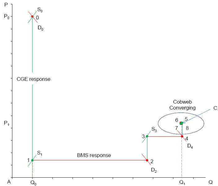
The decreases in the prices of composite goods are then used as exogenous changes in the BMS model, implying that the supply curve in the BMS is a horizontal line through point 1. With a large fall in goods prices, the BMS demand increases to point 2. It should also be noted that household income is also reduced slightly because transfer payments are indexed to the consumer price index (CPI), which decreases with the tariff. Therefore, when goods prices fall, household real incomes fall accordingly. This offsets part of the increase in household demand that is due to the initial fall in prices through a shift of the demand curve.
In the second iteration, the increases in household demands from the BMS model are used to insert exogenous changes to the CGE model. With a new demand curve given by the vertical line through point 2, the same tariff changes result in a less severe fall in the prices of goods in the CGE model than in the first round, so that the supply curve shifts only down to point 3 (from point 0)18. Due to the indexation of transfer payments, household real income is also higher than it was in the previous iteration. With these new price changes, households in the BMS model respond by increasing their demand and pushing the CGE household demand curve horizontally to point 4.
After the first two iterations, the two models enter a familiar cobweb pattern of adjustments (Figure 2b, an enlarged display of the circled area in Figure 2a). After a few more iterations, the two models converge to an equilibrium solution at point C, where the CGE supply curve and the BMS demand curve intersect each other.
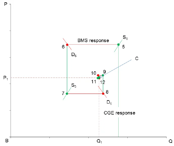
The convergence has two distinct phases. In the first phase, the process follows a single direction, while in the second phase, it follows a cobweb pattern. The first phase involves some realignment of household incomes between the two models. Once the income discrepancies, created by the lagged adjustments between the two models, are reduced to a relatively low level, the cobweb phase begins. The phase of income realignment is crucial for the cobweb convergence. In the above example, the income realignment is achieved without the introduction of a slack variable because the aggregate household saving rate is quite low (only 2.2 per cent of aggregate disposable income according to the survey data). This implies that household expenditures account for almost the entire disposable income in aggregate, so that it is not necessary for the small changes in the saving rate to be transmitted back to the BMS model. This is because the price feedback from the CGE model captures all the changes required for the BMS model to produce a consistent response, including the required adjustments in household income. As a result, the income realignment between the two models can be achieved through the CGE price changes alone, and a slack variable is not required19. It should also be noted that, in this model, the majority of savings comes from the part of capital income that accrues to firms, which is outside the household module and does not rely on the feedback from the BMS model to reach equilibrium. This feature also facilitates the convergence in the iterative simulation process (see Appendix Table A.2 for data details).
Figures 2a and 2b show that convergence is quick and smooth, implying that both models are well-behaved. As Colombo (2010) mentioned, however, a convergent solution may not be a true GE solution due to data or model inconsistencies. To verify whether this solution is a true GE solution the same simulation is conducted with the integrated model. The results from the iterative models are found to be identical to those from the integrated model. This confirms that the iterative approach can be used as an alternative solution method to the integrated approach in this case.
3.2 A not well-behaved case
Not all models are well-behaved. For example, if the saving rate is high, holding the saving rate fixed during the iteration process tends to increase the gap between household disposable income and expenditures and, therefore, lead to diverging solutions. This section will present the case of two linked models that are not well-behaved because the household data imply a large aggregate savings rate.
To demonstrate this case, a different household survey dataset with a higher average saving rate is needed. As the structure of the integrated CGE model is determined by the household data, a different CGE model also needs to be used. The model and database used in this case are taken from another integrated CGE model of the Australian economy, described in Zhang (2015)20. As before, the household module is taken out of the integrated model to be used as a separate BMS model. In the integrated CGE model, the household demands for composite goods are turned off and replaced by the exogenous changes derived from the simulation outcome of the BMS model. Likewise, in the BMS model, the changes in all prices of goods and factors are taken from the simulation outcome of the CGE model.
The simulation is a one-percent increase in the supply of the occupation ‘labourers’ by households in the BMS model. As above, the simulation is first conducted with the integrated model, using a conventional solution method, to produce a set of results to compare with the results from the iterative method.
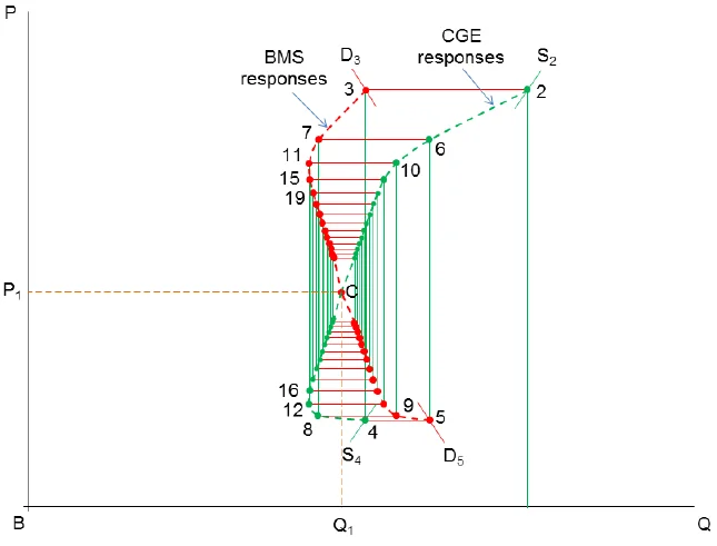
The same experiment is conducted with the two linked models. As in the previous case, the budget balance of the aggregate household in the CGE model is allowed to vary, through endogenous variable H in Equation 1, while saving rates for individual households in the BMS model remain fixed. The iterative interactions between the two models in the aggregate goods markets are plotted in Figure 3a.
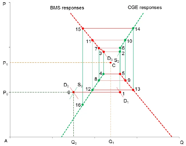
It is clear from the figure that the models are not well behaved. The increase in labour supply causes the quantity responses of the BMS model and the price responses of the CGE model to move away from each other. These diverging responses follow a cobweb pattern and can be seen from the widening gap between the CGE supply curves and the BMS demand curves (these are the small curves that shift at each iteration shown in the figure). The lack of convergence is attributable to a relatively large aggregate saving rate (about 30 percent) in the BMS database, a large initial gap between the aggregate household disposable income and expenditure. If the changes in this gap in the CGE model are ignored by the BMS model, the price feedback from the CGE model alone is unable to align the aggregate household budgets across the two models. Without adjusting saving rates, the income on which the households in the BMS model base their demand decisions would be inconsistent with the income in the CGE model. This inconsistency cumulates over the iteration process and produces the diverging cobweb pattern shown in Figure 3a.
However, the integrated model has already shown that a solution exists, which should be at the centre of the cobweb point C. Now the question is how to induce the two models to reach the observed equilibrium solution at point C. The answer lies in the household saving rate.
To avoid divergence, a simple solution is to swap the endogenous variable H with the exogenous variable
The use of the saving rate as a slack variable allows it to deviate temporarily from its original level in the iteration process. The saving rate needs to be gradually brought back to its initial level in the iteration process. This is achieved by applying a partial adjustment factor (for example, 0.5) to the savings rate changes from the CGE solution, when they are transmitted to the BMS model21. The iteration results for the goods market are plotted in Figure 3b.
As shown in Figure 3a, in the first BMS simulation, with goods prices fixed, an increase in the labour supply increases the demand for composite goods from point 0 to point 1. The first CGE response is an increase in the price from point 1 to point 2. Without the endogenous saving adjustment, the next round of CGE price feedback would induce a quantity response of the BMS model from point 2 to point 3 and lead to a diverging process.
As shown in Figure 3b, with the partial adjustment mechanism, the quantity response in the BMS model is also halved (compare with Figure 3a). As only half of the response of the BMS model is fed back to the CGE model in every iteration, the price responses of the CGE model are also diminishing. The previous cobweb diverging process is therefore replaced by a cobweb converging process. Unlike in Figure 3a, the implied supply and demand curves are now gradually shifted toward equilibrium point C with a diminishing gap, as the household budgets continue adjusting. Finally when the goods market reaches equilibrium at point C, a convergent solution for the two models is reached. This solution is found to be identical to the one obtained with the integrated model. This confirms that the iterative approach has produced the same GE solution as that obtained with the integrated model.
This example shows how the use of the slack variable brings not-well-behaved models to a converging solution. Without a slack variable to adjust the BMS household budgets, the two models would not converge, even though the integrated model showed that such a solution exists.
A slack variable can also be used to solve well-behaved models such as that shown in the first case, but it requires a longer iteration process. This is because the savings adjustment is a slow process. Therefore, if some linked models are known to be well-behaved in iterations, it may be inefficient to use the slack variable approach to find a solution.
4. Revising the BMS model to introduce more flexible functional forms
The household sub-models used above are taken directly from integrated CGE models, in which households have only simple behaviours with given factor endowments. Once the iterative simulation produces the same solution as the integrated model, more flexible structures and complex functional forms, normally unsolvable when embedded in an integrated CGE model, can be readily introduced in the sub-model. No matter how the structure and the behavioural assumptions of the sub-model are modified, so long as they are calibrated to the same initial database, the interactions of both models will still be consistent with each other in iterations, which ensures a convergent and GE solution.
Moreover, to introduce more sophisticated behaviours for economic agents and more realistic policy settings, the sub-model might be written in a format that differs from that used for the CGE model. For example, the sub-model can be written in nonlinear form, or levels, instead of in the percentage change form that is typically used for a CGE model to allow for more flexible functions to be introduced.
This section uses the simple household model, developed in Section 1, as an example to show how such a simple model is converted into a more flexible BMS model and still solvable using the iterative approach. In the following, two examples of modifications are discussed. First, the fixed labour endowment is replaced by a more sophisticated labour supply function. Second, a more complex income tax schedule is introduced. These are the features of the BMS models that might be required to analyse the impacts of changes in income tax policies on individual households or persons. This section also shows that a GE solution is still obtainable for these more complex BMS models if solved with a linked CGE model, using the same iterative approach as above.
4.1 Introducing household labour supply
In the BMS model database, some households have persons who are employed and receive labour income. In the household survey, employment status is classified as “employed”, “unemployed” and “not in the labour force”. The employed are further classified as “full-time” or “part-time”. For each employed person, there is information about their occupation (eight categories), weekly working hours (up to 50 hours) and annual labour income. This rich information in the household survey allows labour supply to be defined at an individual person’s level, as a function of an hourly wage rate22 as well as policy-related factors that affect disposable labour income, such as income tax rates and various transfer payments.
The supply of occupation o by person n in household h is defined as a function of the market wage rate net of personal income tax, as follows (Equation 2),23
where
and, ε(0) is the elasticity of labour supply for occupation 0 with respect to its wage rate,
The labour supply is illustrated in Figure 4. Point E represents an individual’s equilibrium weekly hours worked in a particular occupation at the corresponding hourly post-tax wage rate. The curvature of the supply curve is determined by parameter ε When ε = 1, the labour supply is linear. Lower parameter values produce more curved labour supplies, implying that a labour supply is less responsive to wage changes around E. There is also a maximum number of working hours allowed each week. Once that limit is reached, the supply curve becomes vertical, implying no more response in an individual’s labour supply to further wage increases.
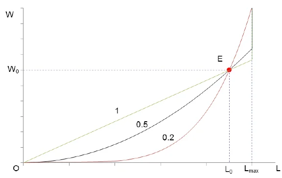
This labour supply responds positively to price signals. However, unlike the functions in a CGE model, this function is truncated at a maximum of 50 hours per week or some specific working hours below 50 for those who are identified as “fully employed”. They are assumed not to respond to further wage increases. Even for those who are close to full employment, a slight rise in wage rate may induce them to hit the limit. Therefore, a rise in wage rate may not necessarily induce an expected rise in labour supply. Such possibilities may cause many conventional solution methods to collapse. The following simulation is used to test if the iterative solution method is flexible enough to handle such complications.
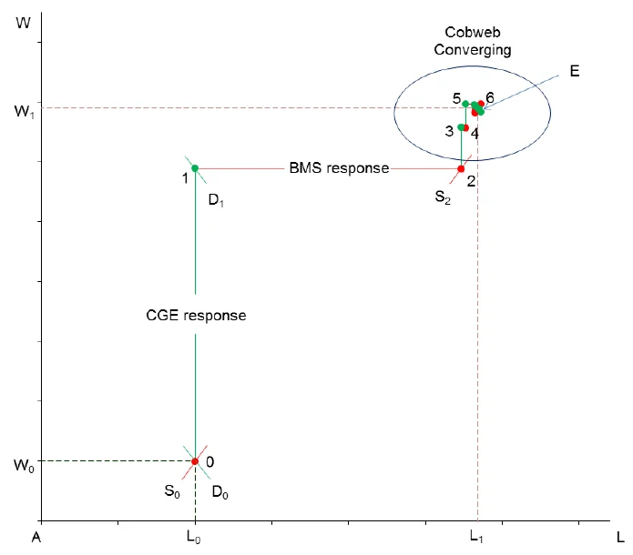
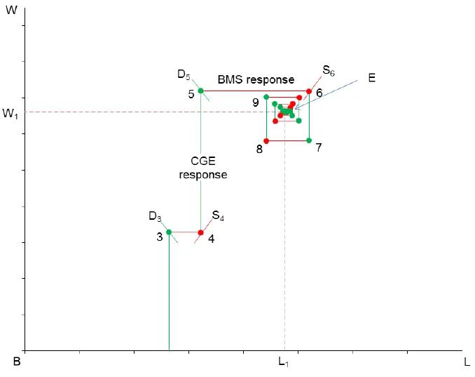
In this simulation, a 10 percent cut in the tariff rates for imports is introduced again in the CGE model. This time, individual persons in the BMS model are able to respond to wage rate changes by altering their labour supply decisions. The labour supply elasticity is set as 0.5 for all occupations. Relative to the previous simulation in which labour supplies were fixed, the introduction of labour supply functions implies more flexible supply-side responses and, therefore, a greater number of iteration may be needed for the two models to converge. That said, in this case, a solution is reached after about eleven iterations.
Figure 5a shows the converging process in the aggregate labour market. As before, the first three simulations realign the household budgets between the two models (Figure 5a) and put the labour-wage interaction on a converging cobweb trajectory (Figure 5b). This example shows that the iterative solution method is flexible enough to accommodate unconventional functional forms so that a GE solution can be reached. More importantly, even if a convergent solution is not found, this method produces temporary solution files that enable the user to track down possible causes of the problem and resolve them by modifying relevant individual behaviours as required.
4.2 Introducing marginal income tax rates
The household survey contains rich information on personal income taxes and various types of transfer payments at the detailed personal and household level. Typically, these tax and transfer payments are not specified in detail in a CGE model because the rules and conditions, on which they are based, are typically too complex to comply with the requirements for solving with a CGE model using conventional solution methods, such as the Johansen approach25.
A separate BMS model, built in levels, provides the flexibility to incorporate the complex rules and conditions of an income tax and transfer system, rather than approximating them with average tax rates as is often seen in CGE models. In the second example, a detailed income tax schedule is incorporated in the labour supply function, introduced above, to illustrate how a BMS model with these complex tax rules is solved in levels iteratively with a CGE model, which is solved with linear algebra.
Australia has a progressive income tax system. There are five marginal tax rates, applied to different income ranges, as shown in Table 1. The household survey data also reports the amounts of income tax each person paid, which accounts for deductions and other idiosyncrasies of the tax system.
| Income range ($) | Initial tax rates (%) | Simulated changes (%) | New tax rates (%) |
|---|---|---|---|
| 0 - 18,200 | 0 | 0 | 0 |
| 18,201 - 37,000 | 19 | 5 | 19.95 |
| 37,001 - 80,000 | 32.5 | 5 | 34.13 |
| 80,001 -180,000 | 37 | 10 | 40.70 |
| 180,001 and above | 45 | 10 | 49.50 |
Source: Australian Taxation Office (https://www.ato.gov.au/rates/individual-income-tax-rates/accessed 1 April 2016) and author calculations.
In the BMS model, the reported income tax
This equation shows that the observed income tax is defined as the sum of the estimated tax plus a residual
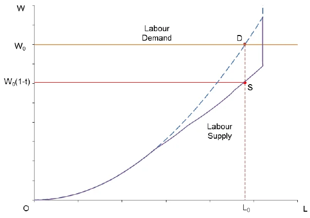
The impact of income tax on the labour supply of a particular person is illustrated in Figure 6. The ‘tax free’ labour supply curve intersects the horizontal labour demand curve (at the wage rate paid by the firm) at point D. The income tax schedule shifts the worker’s supply curve down to point S. The observed market wage rate is W0 and the associated labour supply is L0. This person’s taxable income is given by the area OW0DL0. The income tax is paid according to a set of progressive marginal rates. This person’s after-tax wage rate is therefore equal to W0(1 – t), where t is the income tax rate, derived from the total tax paid and the total taxable income. For a given wage rate, a change in any tax rate alters the implied average income tax rate and the aftertax wage rate, and therefore, induces a change in labour supply26.
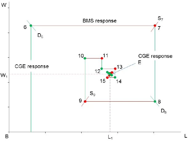
In this section, the income tax schedule is assumed to change according to the exogenous changes that produce the new tax rates in the last column of Table 1. This BMS model is solved iteratively with the same CGE model used above. The process of convergence in the labour market is shown in Figure 7a with the final stages enlarged in Figure 7b. The increase in income tax in the BMS model reduces the post-tax wage rate and decreases labour supply. With the market wage fixed, the total labour supply in the BMS model moves along a horizontal demand curve from point 0 to point 1, indicating a fall in labour supply. With such a reduced labour supply imposed in the CGE model, the market wage tends to rise, which increases labour costs for firms and reduces their demand for labour, as shown in the vertical shift of labour demand up to point 2 in Figure 7a. As before, after realigning household budgets between the two models in the first two iterations, the simulations enter the cobweb stage, converging toward equilibrium E.
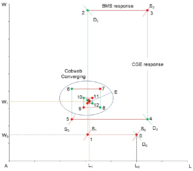
This example shows that the introduction of conditional functional forms and progressive marginal tax rates is not an obstacle to convergence. This is because the discrete functions and complex rules are implemented at individual or household levels. When they are aggregated to the national level to be transmitted to the CGE model, the detailed discontinuities largely cancel out, so in this case, the BMS aggregations in the CGE model are still “well-behaved”, and, therefore, the solution is easy to find.
4.3 A note about tractability and solution time
As the sub-model is outside the CGE model structure, the solution time for solving a sub-model and its linked CGE model can be substantially reduced, compared with an integrated model. Take the first experiment of tariff reduction, presented in this paper, as an example. With an Intel Core i5 computer, it takes the GEMPACK software 3 minutes and 44 seconds to produce a Johansen solution for the integrated CGE model. Using the iterative approach and combining the two models in one TABLO code27, it takes only 3 seconds for the CGE model to produce a Johansen solution and the BMS model to produce a response file. If ten iterations are required for a convergent solution, it still takes only 30 seconds to complete, a substantial gain in computing time, especially when multiple experiments are required in a project. The difference in solution time arises because the large BMS model is treated as a data processing task, rather than as part of the large simultaneous equation system that describes the CGE model; this means that the matrix to invert remains small despite the large number of households in the BMS model.
5. Some concluding remarks
This paper sought to “wrap” a CGE model around a BMS model to improve policy analysis by accounting for potential GE effects. The proposed approach started with an integrated CGE model to show how part of the model could be separated to from a sub-model, and still be solved within the GE framework, using an iterative simulation method. Compared with conventional CGE solution methods, the iterative approach is more flexible and provides an alternative way of introducing sub-models with complex functional forms and behavioural assumptions that are not normally solve-able in CGE models.
The key to this iterative approach is threefold. First, the database of the sub-model must be fully consistent with that of the CGE model. Second, the model theories must not overlap and should complement each other exactly. Third, to induce the iterative process to converge, a slack variable may be needed in some cases. In this paper, the saving rate in the CGE model is used as the slack variable to realign the household budgets in the BMS model so that their aggregate response is consistent with the budget constraint implied by the CGE model.
Although the approach is applied to the household module in this paper, the principles that underlie the method could apply to other parts of a CGE model. To some extent, the household sector may be easier to separate out than some of the industry sectors because its links with the rest of the CGE model are relatively simple, but the principles discussed here are likely to be useful in decomposing an industry sector from a CGE model and solve the two models iteratively. A separate industry PE model could be useful for introducing those industry-specific features that are difficult, if not impossible, to be incorporated into a CGE equation system. This may lead to a more flexible modelling framework, better adapted to addressing specific policy questions at sub-sectoral levels, while accounting for GE effects if required28. This could be an important area for further research.
Footnotes
1.
There is extensive literature covering each area. See, for example, the surveys by Figari, Paulus, and Sutherland (2007) on income distribution studies and a survey article on CGE-microsimulation modelling by Ahmed and O’Donoghue (2007).
2.
Early examples can be found in Dixon, Malakellis, and Meaghe (1996) and Polette and Robinson (1997), who link a MS model, STINMOD, developed by NATSEM, with a CGE model, MONASH, developed by the Centre of Policy Studies, to simulate the impacts of microeconomic reforms on the distribution of incomes across Australian households.
3.
The iterative approach was popular in solving so-called applied general equilibrium (AGE) models, pioneered by Scarf (1973) in the 1970s. However, the AGE model was superseded by the CGE model in the 1980s, as the latter was able to provide relatively quick solutions for large computable GE models for a whole economy. The iterative approach proposed in this paper is related conceptually to the early approaches. Unlike those approaches, however, in this paper, the CGE model is solved via more efficient linear algebra techniques.
4.
Savard (2003, footnote 8 on page 8) finds that “convergence was difficult with using the ‘Almost Ideal Demand System”.
5.
Rutherford (1999) discusses the problems associated with what “in many settings […] is known as the problem of exact aggregation” (p.2), which occurs when two models that are interacting take different views of how household behaviour is determined. He also discusses conditions under which “the demand function[s] describing a set of heterogeneous consumers can be replaced by the demand for a single agent”. As will be shown below, this “problem of exact aggregation” does not arise in the context of this paper, because the individual functions are not aggregated into a single function. Rather, the optimal quantities from each household from the BMS model are aggregated to use as exogenous changes for a CGE model, in which the aggregate consumption function is omitted by design.
6.
Savard and Annabi (2004) propose a checklist to help find a convergent solution with the TD-BU approach.
7.
See, for example, Cogneau, and Robillard (2001); Cockburn (2006); Cororaton and Cockburn (2007); Cockburn et al. (2008).
8.
For example, the theory and properties of a PE model may imply multiple equilibria. This would make it impossible to find a GE solution, certainly using standard Johansen solution methods.
9.
Böhringer and Rutherford (2006) propose a similar approach, which decomposes an energy model from an integrated MCP (Mixed Complementarity Programming) model. This approach “puts strong emphasis on overall economic consistency and therefore makes use of a single integrated modelling framework in order to ‘hard-link’ bottom-up and top-down features”. (Böhringer & Rutherford, 2006, p.1)
10.
The simple CGE model is similar to the ORANI-style models developed at the Centre of Policy Studies.
11.
Although the preferences of the representative consumer in the original CGE model and of each household in the extended model are both Cobb-Douglas, the consumption shares for each household are different, making the aggregation into a single representative function non-trivial and the responses from the multiple household specification is different from the response that would arise from a single representative household specification.
12.
We use the expression BMS to identify the household module even though at this stage of the paper it might not look very different from a disaggregated household module in any other CGE model. In this context, the BMS consists of many households, each of which makes decisions on the consumption side, based on a continuous, well-behaved individual (Cobb-Douglas) utility function, with fixed labour and capital endowments. This is relaxed in Section 3, where the household module is replaced by a more conventional BMS with discrete choices in terms of labour supply and step-wise increasing marginal income tax rates.
13.
In this way, the theory of the two models does not overlap but complement each other strictly. Some might argue that this is not a “complete” CGE model, because it does not account for consumer behaviour. Another way to look at this version of the CGE model is that it produces a solution for other sectors subject to consumer demands. In this way, excising consumer demand is akin to adopting some simple closure rule for other parts of a CGE model such as government expenditure or the trade balance.
14.
For example, CAPITA-B, a BMS model that accounts for most of the characteristics of the Australian tax and transfer system and is in use in several Australian Government departments. Marshall (2016) developed a platform and policy parameters (e.g. tax rates, transfer eligibility criteria and taper rates, etc. are updated annually).
15.
GEMPACK is a suite of economic modelling software developed by the Centre of Policy Studies, Victoria University, Australia.
16.
This list includes all variables and equations that are required to solve for the GE solution, but does not include variables and equations that are used exclusively for presentational purposes, such as those for aggregating quantities or averaging prices. The reporting variables can be added to the models without affecting its solution.
17.
More explanations about the use of saving rate as a slack variable will be given in the second example in Section 2.
18.
In the context of this paper, the “iteration” is a process of tâtonnement, which does not involve updating the databases. In each round, new exogenous changes are applied to the initial database, that is, each model tests its responses to a new set of exogenous changes from its counterpart until the two equilibrium solutions converge. In the CGE model, for example, the tariff reductions are repeated with a new set of
quantity changes from the BMS model until all prices reach equilibrium. The different points in the figures show the different solutions that are obtained from different combinations of the policy change and each new price or quantity changes that are tested, until the equilibrium is reached.
19.
If the aggregate saving rate is zero, changes in household disposable income in the CGE model must always be consistent with changes in expenditure, because all changes in prices and quantities that produce the new equilibrium are consistent with changes in income and expenditure aggregates. In such a case, there is no need for a slack variable because there is no discrepancy between household income and expenditure.
20.
This model predates the well-behaved model shown in the first case and characterises the Australian economy in the early 1990s when the aggregate household savings implied by the household survey was larger.
21.
The author is grateful to Maureen Rimmer for pointing out that Dixon, Pearson, Picton and Rimmer (2005) use a similar partial adjustment approach in a different context: to facilitate convergence when solving the MONASH model under rational expectations.
22.
The wage rate is derived from labour income and hours worked as reported in the household data. For the unemployed, this (reservation) wage is imputed as the wage rate for “labourer”.
23.
For this illustration, only income tax is selected as a policy variable in determining labour supply behaviour. Although included in the model and database, other policy variables such as transfer payments are assumed to be fixed and therefore not to affect labour supply.
24.
Alternatively, individuals’ labour supply behaviour could be specified as a result of a utility maximisation problem as, for example, in the CAPITA-B model (Marshal 2016). While this would increase solution time, it does not affect the principles presented here.
25.
It may be possible to use some other more sophisticated methods to solve these models, but the approach advocated here demonstrates that this may not be necessary.
26.
This is a common specification in microsimulation models where labour supply is a function of after-tax income, including transfers, rather than a function of wages. An alternative specification might be that the labour supply is determined by the marginal tax rate. In such a specification, any changes in inframarginal tax rates do not affect labour supply. By contrast, linking labour supply to marginal changes in after-tax income means that a change in any of the tax rates changes the amount of tax owed and labour supply.
27.
See Appendix A for an effective GEMPACK implementation.
28.
It is worth noting that the approach is facilitated by using a simple CGE structure. For example, the principles could be used to link MARKAL-type energy models with a simple CGE structure.
Appendix
A. A simple approach to iterative simulations for gempack users
GEMPACK users can write the CGE model in percentage changes and the sub-model in levels in a single TABLO code. The CGE model is defined in the normal way using “VARIABLE” and “EQUATION” statements, while the BMS model is defined using “COEFFICIENT” and “FORMULA” statements in a separate section.
The CGE model is run first to produce a solution file. Those variables that are used as input into the BMS model, such as goods and factor prices, are written to a Header Array (HAR) file using the SLTOHT command. The sub-model then reads in the CGE shocks from this HAR file and writes its results to another HAR file to be used as exogenous changes in the CGE model in the next iteration. A batch file can be used to automate the procedure so that, in each simulation, the two models can run in sequence and also produces an input file for the next iteration.
This approach allows the BMS model to be written in levels within the same code as the CGE model. Therefore, more complex functional forms, such as conditional or discrete functions, and unconventional behavioural assumptions, such as switching between different options, can be implemented alongside a linearised CGE equation system, which can save significant computation time.
B. The database of an integrated model
The model is built on the basis of Australian input-output table 2012–13 (Australian Bureau of Statistics, 2015) and the 2009–10 Household Expenditure Survey (HES) and Housing and Income Surveys (HIS) (Australian Bureau of Statistics, 2012). The input-output table includes 104 industries and two factors of production, labour and capital. An aggregated version of this table is shown in Table B.1.
| 1 ind | 2 hou | 3 gov | 4 inv | 5 stk | 6 exp | 7 mgn | Total | |
|---|---|---|---|---|---|---|---|---|
| 1 dom | 1,159,672 | 566,012 | 265,156 | 327,917 | −2,034 | 270,578 | 272,793 | 2,860,094 |
| 2 imp | 167,734 | 79,915 | 2,878 | 63,035 | 3,387 | 316,949 | ||
| 3 mgn | 94,733 | 127,542 | 2,672 | 20,227 | −87 | 27,706 | 272,793 | |
| 4 GST | 3,624 | 37,415 | 0 | 8,235 | 0 | 1,090 | 50,364 | |
| 5 tax | 17,831 | 25,502 | 0 | 13,609 | 652 | 0 | 57,594 | |
| 6 sub | −6,636 | −5,463 | 0 | −1,154 | −14 | −616 | −13,883 | |
| 7 fac | 1,371,108 | 1,371,108 | ||||||
| 8 ptx | 52,028 | 52,028 | ||||||
| Total | 2,860,094 | 830,923 | 270,706 | 431,869 | 1,904 | 298,758 | 272,793 | 4,967,047 |
Notes: Basic values of imports (316,949) include import tariffs (3,233).
Source: Compiled from Australian National Accounts: Input-Output Tables, 2012–13 (ABS 5209.0.55.001).
Industries (aggregated in the first column) use domestically produced and imported intermediate goods in production. Domestically produced goods (the first row) are used as intermediate inputs into current production by industries and other users: a representative household as consumer and investor, and government. Some products are exported, and some are used as transport margins, which are added to the basic price of products. The total costs of domestic outputs (the sum of the first column) is equal to the total sales of domestic products (the sum of the first row).
As the owner of primary factors, the household receives factor incomes. Household primary income is divided between consumption expenditure and savings. Government collects various taxes and uses this income to pay for expenditures on goods and services.
Investment is partly funded by domestic savings. The gap between investment and saving is net foreign investment (NFI) inflow (18,191), which is equal to the trade deficit (316,949 – 298,758).
The data on household income and expenditure are extracted from the 2009–10 HES and SIH (ABS, 2011). The HES-SIH data are contained in two unit record data files: one file contains expenditure data on 9,774 sample households; the other file contains data on income sources for the 17,919 individual members of the sample households. The household data are mapped to the income sources and commodity categories of the CGE model.
On the income side, HES-SIH income items are aggregated to 33 types of personal income items: wage incomes from 8 labour occupations, capital income, 23 government benefits, and income taxes. In households with multiple income earners, incomes from each source are consolidated within each household. Table B.2 displays the allocation of the HES-SIH sources of income to the CGE database items.
| CGE model | Household Expenditure Survey (HES-SIH) | |
|---|---|---|
| Wages for eight occupations (same as those in HES-SIH) | Managers and administrators; | Clerical and administrative workers; |
| Professionals; | Sales workers; | |
| Technicians and trade workers; | Machinery operators and drivers; | |
| Community and personal service workers; | Labourers; | |
| Capital | Own unincorporated business; | Superannuation/Annuity/Private pension and other regular sources |
| Investment; | ||
| Transfer payments from government | Austudy/Abstudy | Partner allowance |
| Age pension | Service pension | |
| Carer allowance | Sickness allowance | |
| Carer payment | Special benefit | |
| Disability pension | War widows pension | |
| Disability support pension | Widow allowance | |
| Family tax benefits | Wife pension | |
| Newstart allowance | Youth allowance | |
| Other pensions and allowances | Utilities allowance | |
| Overseas pensions and benefits | Senior supplement | |
| Parenting payment | Pension supplement | |
| Baby bonus payment; | ||
| Direct taxes | Income taxes | |
Source: Australian Bureau of Statistics, 2012.
On the expenditure side, there are 614 items recorded under the Commodity Code (ComCode) system in the HES data file. Among them, 485 can be aggregated into corresponding commodities in the input-output table. The rest need to be allocated to more than one commodity in the input-output table. In the absence of additional information about the composition of these commodities, the value shares of the commodities in the input-output table are used to allocate expenditures on these items.
Once the preliminary processing of the HES data is complete, a five-step procedure reconciles the differences between the two databases (Zhang, 2015). As the HES expenditure and income data are expressed in purchaser prices, they are aligned with input-output data in purchaser prices. The five steps are:
Use the HES weights to inflate the sample household data to the value for the whole population.
Scale the aggregated HES expenditure to be consistent with the total household expenditure in the input-output table.
Use the same scaling factor to scale the aggregated HES primary incomes.
Adjust each HES household’s expenditure shares, while keeping total expenditure on each product constant, so that the aggregation of all HES expenditures is consistent with the commodity consumption pattern of the representative household shown in the input-output table.
In each industry in the input-output table, adjust factor income shares (labour by occupation and capital), while keeping the total value of factor income constant, so that the aggregated labour and capital income (net of capital savings) in the input-output table are consistent with the aggregated labour and capital incomes in the household data.
The aim of the second and third steps is to preserve the original relativities between households in the survey data. The aim of the fourth and fifth steps is to keep the budget balances of individual households and the factor returns of individual industries in the input-output table unchanged. A bi-proportional adjustment technique, such as RAS, or an entropy-based method, is required to carry out the last two steps.
A comparison between factor income in the 2012–13 input-output table and household income in the 2009–10 HES-SIH data is shown in Table B.3. A scaling factor of 1.3634 is used to update the 2009–10 HES-SIH data to the level consistent with the 2012–13 input-output table.
| CGE data | HES-SIH scaled | HES-SIH | |
|---|---|---|---|
| (1) | (2) | original | |
| Expenditure | 830,924 | 830,924 | 609,468 |
| Income | 1,371,109 | 850,486 | 623,816 |
| Labour income | 744,282 | 744,282 | 545,918 |
| – Managers & administrators | 132,202 | 132,202 | 96,968 |
| – Professionals | 229,510 | 229,510 | 168,341 |
| – Technicians & trade workers | 101,273 | 101,273 | 74,282 |
| – Community & personal service | 45,706 | 45,706 | 33,525 |
| – Clerical & administrative workers work s | 91,417 | 91,417 | 67,052 |
| – Sales workers | 43,234 | 43,234 | 31,712 |
| – Machinery operators & drivers | 50,821 | 50,821 | 37,277 |
| – Labourers | 50,118 | 50,118 | 36,761 |
| Capital income | 626,826 | 154,400 | 113,250 |
| Benefits (23) | 106,875 | 78,391 | |
| Income Tax (-) | 155,071 | 113,742 | |
| Savings | 540,185 | 19,562 | 14,348 |
Notes: 1. Capital income in the input-output table is divided between household (154,400) and firm saving (472,426). 2. Scaling factor between columns (2) and (3) = 1.3634.
C. The model structure
The core equations of the model are provided in this section, which is followed by a brief discussion of the model’s theoretical structure. The sets used in the model equations are listed as follows.
Demands for domestic and imported goods (Equations A1–A10)
Domestic price of imported good c, exclusive of duty
where ex is the nominal exchange rate (domestic currency value per unit of foreign currency), and
Basic price of good c from source s for user u
where
CES demand of user u for good c from source s (exclusive of stk)
CES price for composite good c for user u
Demand of good c for user u for margin good m
Producers’ price of composite good c for user u
Purchasers’ price of composite good c for user u
where
Producers’ price of exported good c
Foreign demand for exported good c
where
Foreign price of exported good c
where
Final user incomes and demands for composite goods (Equations A11–A18)
Household factor income
where scap is the share of capital income firms retain for investment.
Household disposable income
Expenditure income of final user u
where sgov is government saving rate and
where
Net foreign direct investment (in domestic currency)
where Qfdi is the real inflow of net foreign direct investment. Purchasers’ price index for user u
Demand of user u for composite good c
where X(u) is the output of industry u and Q_s(c,“gov”) and Q(c,“stk”,s) are exogenous variables.
Budget constraint for government and inventory
Industry outputs, prices and demands for factors (Equations A19–A28)
CES demand of industry i for labour occupation 0
where
Basic price of factor f in industry i
where
CES demand of industry i for factor f
where
CES price index for composite factor in industry i
Unit cost of output in industry i
Basic price of output in industry i
where
Total supply of labour occupation o (equal to its demand in equilibrium)
Total supply of capital (equal to its demand in equilibrium) (⇒Pcap)
Industry supplies of multi-products (Equations A29–A32)
CET supply of good c from industry i
CET price index for composite goods (equal to
Total supply of good c from all industries
Total sales of good c (equal to
Household income and expenditure (Equations A33–A38)
Factor income from factor f for person n in household h
where
Taxable income for person n in household h
where
Disposable income for person n in household h
where
Expenditure income for household h
Changes in saving rate for household h
Demand of household h for composite good c
Linking household variables with CGE aggregates (Equations A39–A43)
Aggregation of household supplies of capital stock
Aggregation of household supplies of labour occupation o
Aggregation of household demands for composite good c
Average household income tax rate
Aggregation of household real benefits
| Sets | Definitions |
|---|---|
| COM(1,…,m): | Commodities (indexed by c) |
| IND(1,…,m): | Industries (indexed by i) |
| MCM(1,…,n): | Margin commodities (indexed by m) |
| NCM(= COM - MCM): | Non-margin commodities (indexed by c) |
| FUSR(gov, hou, inv, stk): | Final users of commodities (indexed by u) |
| USR(=IND + FUSR): | Users of commodities (indexed by u) |
| USR_stk(=USR - stk): | Users of commodities, exclusive of stk (indexed by u) |
| SRC(dom, imp): | Domestic/import sources of commodities (indexed by s) |
| FAC(lab,cap): | Factors of production (indexed by f) |
| OCC(1,…,8): | Labour occupation (indexed by o) |
| SAV(inv,stk): | Saving destination (indexed by s) |
| HOU(1,…,9774): | Sample households (indexed by h) |
| PER(1,…,6): | Persons in a household (indexed by p) |
| B23(1,…,23): | Transfer payments (indexed by b) |
| TAX(GST, tax, sub): | Three tax items (indexed by g) |
The model specifies the behaviours of three types of economic agents:
A representative firm in each industry, which purchases intermediate inputs and factor services to produce goods or services. For given demand for its products and input prices, the firm uses constant-return-to-scale (CRTS) technology to minimise the costs of production.
A household sector, which plays three roles: as factor owner, it receives factor incomes from firms; as consumer, it spends income on goods and services to maximise its utility; and as investor, it allocates savings to form new capital.
A government sector, which collects revenue from taxes on goods and services and from household and spends income on transfers to households and on purchasing goods and services.
The price system consists of three layers:
Basic price = unit cost of production, including intermediate and factor input costs, plus production tax; the basic price of imported goods include import tariffs.
Producer price = basic price plus transport and sales margin services.
Purchaser price = producer price plus indirect taxes.
The basic structure of the model can be summarised in the behaviours of two groups of users: users of intermediate inputs (firms) and users of final products (household, government and investor).
Firm behaviour has five components (refer to Table B.1).
Industry demand for domestic and imported intermediate inputs: a CES cost-minimising demand function of two variables – the given purchasers’ prices and the industry demand for the composite good (Equation A3).
Industry demand for composite intermediate inputs: a Leontief cost-minimising demand function of the industry’s firms (Equation A17).
Industry demand for factor inputs: a CES cost-minimising demand function of two variables -basic factor prices and the industry’s output (Equations A19–A23).
The input-output table used for this model is a product-industry table, where some industries produce multiple products. To model this production structure, a CET supply of multiple products is introduced in each industry (Equation A29), which is a function of the industry’s total output, X(i), and the basic prices of the products produced, P(c,“dom“). The general equilibrium output of each industry X(i) is determined by linking the associated CET price index with the basic price of the industry
Final users’ behaviours (household, government and investor) have three components.
Final user’s demand for domestic and imported goods (Equation A3): a CES cost-minimising demand function of two variables – the given purchasers’ prices and final user’s demand for the composite good.
Final user’s demand for composite goods (Equation A17): the functional form varies depending on the final user concerned. For investors, it is a Leontief cost-minimising demand function of capital formation. Government demand is assumed to be exogenously given. For households, it is an aggregation of individual household demands to be defined in the household module below.
Final users’ income and expenditure (Equation A13): as indicated earlier in the model data section, the three final users all have their expenditures fully paid for by their respective incomes, and, therefore, all have balanced budgets.
As government and inventory demands are exogenously given, two budget constraints are required, so that government saving rate sgov and household saving rate for inventory
The foreign demand for exported goods is defined in a constant elasticity of demand function (Equation A9).
There are two components in the household module, specified in Equations A33 to A38. On the income side, each person’s incomes from various sources are aggregated within a household. Four types of income are defined.
Factor income, composed of labour income from different occupation categories and from capital (Equation A33).
Taxable income, composed of factor income plus various benefits received from the government and transfer income from other households, as derived from the HES-SIH datasets (Equation A34).
Disposable income, defined as taxable income, net of income tax (Equation A35).
Expenditure income, referring to the part of household disposable income that is used for current consumption (Equation A36). The remainder is household saving, which is assumed to be adjusted by changes in the average saving rate
(Equation A37).
On the expenditure side, household demands for the composites of domestically produced and imported goods are derived from a Cobb-Douglas utility function, which is a function of household income and goods purchaser prices (Equation A38). As household incomes and consumption patterns (which determine the parameters in the demand functions) are different, each household has a unique and individual response to a given set of price changes. This functional form is chosen for simplicity consideration. Other more flexible functional forms may also be used, but are unlikely to alter the model’s convergence behaviour.
Household factor endowments can be aggregated and linked to the variables of factor supplies in the main model (Equations A39–A43). The household supplies of factors are assumed to be fixed in the integrated model. This assumption is relaxed when using a separate BMS model in Section 3 of this paper.
In this model, the following variables are set as exogenous
All tax rates and real benefits:
and Household and firm saving rates:
and scap Household supplies of capital and labour:
and The world prices of imports, foreign income and net foreign investment:
and Qfdi Foreign exchange rate ex, which is also used as the numeraire
Other variables are all endogenously defined by an equation, except the following three groups of variables, which are not defined by any equation.
Government saving rate sgov and household saving rate for inventory
Industry output X(i) and product basic price P(c,“dom”)
Basic prices for labour (by occupation)
and capital Pcap
The equilibrium values of first two groups of variables are determined by Equations A18, A30 and A32, respectively, which have been discussed above, not to be repeated here. The basic prices of labour and capital are determined by their respective market clearing conditions given in Equations A27 and A28.
As a result, the model has equal numbers of endogenous variables and equations, implying a valid closure and a unique solution. A test simulation confirms that this is the case.
References
- Aaberge, R, Colombino, U, Holmøy, E, Strøm, B, Wennemo, T (2007). Population ageing and fiscal sustainability: integrating detailed labour supply models with CGE models. In Harding, A, Gupta, A (Eds.), Modelling Our Future: Social Security and Taxation (pp. 259–290). Amsterdam: Elsevier.
- Ahmed, V, O’Donoghue, C (2007). CGE-microsimulation modelling: a survey. MPRA Paper 9307. CGE-microsimulation modelling: a survey. MPRA Paper 9307.
- Arntz, M, Boeters, S, Gürtzgen, N (2005). Alternative Approaches to Discrete Working Time Choice in an AGE Framework, ZEW Discussion Papers. Alternative Approaches to Discrete Working Time Choice in an AGE Framework, ZEW Discussion Papers.
- Arntz, M, Boeters, S, Gürtzgen, N, Schubert, S (2006). Analysing welfare reform in a microsimulation-AGE model: the value of disaggregation. .
- (2012). Household Expenditure Survey and Survey of Income and Housing 2009-10.
- (2015). Australian National Accounts: Input-Output Tables, 2012-13.
- Böhringer, C, Rutherford, T (2006). Combining Top-Down and Bottom-up in Energy Policy Analysis: A Decomposition Approach. ZEW Discussion Paper No. 06-007. Combining Top-Down and Bottom-up in Energy Policy Analysis: A Decomposition Approach. ZEW Discussion Paper No. 06-007.
- Bourguignon, F, Savard, L (2008). The Impact of Macroeconomic Policies on Poverty and Income Distribution: Macro-Micro Evaluation Techniques and Tools.
- Cockburn, J (2006). Trade liberalisation and poverty in Nepal: a computable general equilibrium micro simulation analysis. In In Bussolo, M, Round, J (Eds.), Globalization and Poverty: Channels and Policies (pp. 171–194). London: Routledge.
- Cockburn, J, Corong, E, Cororaton, C (2008). Poverty effects of the Philippines’ tariff reduction program: insights from a CGE model. Asian Economic Journal, 22, 287–317.
- Cockburn, J, Savard, L, Tiberti, L (2014). Handbook of Microsimulation Modelling.
- Cogneau, D, Robillard, AS (2001). Growth distribution and poverty in Madagascar: learning from a microsimulation model in a general equilibrium framework. TMD Discussion Paper 61. Growth distribution and poverty in Madagascar: learning from a microsimulation model in a general equilibrium framework. TMD Discussion Paper 61.
- Colombo, G (2010). Linking CGE and microsimulation models: a comparison of different approaches. International Journal of Microsimulation, 3, 72–91.
- Cororaton, C, Cockburn, J (2007). Trade reform and poverty-lessons from the Philippines: a CGE microsimulation analysis. Journal of Policy Modeling, 20, 141–163.
- Dixon, P, Malakellis, M, Meagher, T (1996). A microsimulation/applied general equilibrium approach to analysing income distribution in Australia: plans and preliminary illustration. Preliminary Working Paper No. IP-67. A microsimulation/applied general equilibrium approach to analysing income distribution in Australia: plans and preliminary illustration. Preliminary Working Paper No. IP-67.
- Dixon, PB, Pearson, KR, Picton, MR, Rimmer, MT (2005). Rational expectations for large CGE models: A practical algorithm and a policy application. Economic Modelling, 22, 1001–1019.
- Figari, F, Paulus, A, Sutherland, H (2007). Microsimulation and policy analysis. In Atkinson, AB, Bourguignon, F (Eds.), Handbook of Income Distribution (pp. 2142–2221). Amsterdam: Elsevier.
- Fredriksen, D, Heide, KM, Holmoy, E, Solli, IF (2007). Macroeconomic effects of proposed pension reforms in Norway. In Harding, A, Gupta, A (Eds.), Modelling Our Future: Social Security and Taxation (pp. 107–142). Amsterdam: Elsevier.
- Marshall, D (2016). CAPITA-B: A Behavioural Microsimulation Model. Canberra: Staff Research Note, Productivity Commission.
- Polette, J, Robinson, M (1997). Modelling the impact of microeconomic policy on Australian families. Discussion Paper 20. Modelling the impact of microeconomic policy on Australian families. Discussion Paper 20.
- Rutherford, T (1999). Sequential joint maximization. In Weyant, J (Ed.), Energy and Environmental Policy Modeling (pp. 135–179). New York: Springer.
- Rutherford, T, Tarr, D, Shepotylo, O (2004). Poverty effects of Russia’s WTO accession: modelling ‘real’ households and endogenous productivity effects. World Bank Policy Research Working Paper 3473. Poverty effects of Russia’s WTO accession: modelling ‘real’ households and endogenous productivity effects. World Bank Policy Research Working Paper 3473.
- Savard, L (2003). Poverty and income distribution in a CGE-household micro-simulation model: top-down/bottom up approach. Working Paper 03-43. Poverty and income distribution in a CGE-household micro-simulation model: top-down/bottom up approach. Working Paper 03-43.
- Savard, L, Annabi, N (2004). Note on convergence problems with large CGE microsimulation models.
- Scarf, H (1973). The Computation of Economic Equilibria. New Haven: Yale University Press.
- Zhang, X-G (2015). Incorporating household survey data into a CGE model. .
Article and author information
Author details
Acknowledgements
The author is grateful to Patrick Jomini, Larry Cook, John Salerian, audiences at presentations held at the Productivity Commission, the 19th Annual Conference on Global Economic Analysis, Washington, DC., June 15–17, 2016 and the National CGE Workshop in Canberra, August 8, 2016, and three anonymous referees for their helpful comments. The views expressed here are the author’s only and do not necessarily reflect those of the Productivity Commission.
Publication history
Copyright
© 2017, Zhang
This article is distributed under the terms of the Creative Commons Attribution License, which permits unrestricted use and redistribution provided that the original author and source are credited.