Global sensitivity analysis of a model simulating an individual’s health state through their lifetime

Abstract

In public health, model predictions are used by decision-makers to minimise health burdens and monetary costs of non-communicable diseases. Fully understanding the uncertainty underlying those predictions is thus crucial. One-parameter-at-a-time methods are typically used for model uncertainty analysis but are often impractical for large-scale nonlinear models containing a very large number of parameters and cannot be used to examine the uncertainty associated with parameter interaction. An individual-based chronic disease model was developed to model the impact of Body Mass Index (BMI) trends on the rates of non-communicable diseases. The model was simulated for overweight and obese male case studies and used to predict their life expectancy, disease-free life expectancy and quality-adjusted life years. Uncertainty was estimated by carrying out a global sensitivity analysis by assessing the contribution to the overall uncertainty from a selection of parameters individually and from their interactions. Results show that the uncertainty of the BMI input parameter had the greatest impact on the disease-free life expectancy and quality- adjusted life year uncertainty compared to the relative risks of colorectal cancer and stroke. Life expectancy uncertainty was influenced by BMI and colorectal cancer relative risks. Global sensitivity analysis enables the assessment of the parametric uncertainty for individual parameters and their interaction. This allows the communication of the uncertainty of different policy options. A strategy for scaling-up uncertainty analysis from an individual to a population level is discussed.

1. Introduction

Microsimulation models are becoming increasing popular in public health (Atella, Belotti, Carrino, & Piano Mortari, 2017; Goldman et al., 2009; Gonzalez-Gonzalez, Tysinger, Goldman, & Wong, 2017; Hennessy et al., 2015; Hunt et al., 2017; McPherson, Marsh, & Brown, 2007; Rogers et al., 2014). These models have been used to predict the future epidemiological and economic impacts of risk factors (e.g. Body Mass Index (BMI), smoking, alcohol consumption) on rates of non-communicable diseases in a given population (Ahern et al., 2017; Hunt et al., 2017). Typically these models simulate the health profile of between 5,000 and 100 million individuals. Due to the increasing availability of health-related ‘big’ data and computing power, these models are becoming increasingly more complex and data driven. Model input data are commonly extracted from multiple sources each with varying levels of uncertainty. In general, a quantification of the uncertainty of outputs from public health microsimulation models is not analysed. Uncertainty estimates of model outputs which reflect the uncertainty of the model input parameters are important to include because they provide more detail about the confidence of these outputs (Mathijssen, Petersen, Besseling, Rahman, & Don, 2008).

There are two main methods for analysing the parametric uncertainty of complex models such as microsimulation: deterministic and probabilistic (there is another method which uses fuzzy mathematics but it is not as widely used). Deterministic analysis considers fixed variation in parameter values whereas probabilistic analysis considers random variations in parameter values. Local deterministic sensitivity analysis such as one-at-a-time can be used to analyse the impact of the uncertainty from one input parameter on the model output (Saltelli, 1999). However, these methods are unrealistic for models with many complex interactions and with a large number of input parameters. Probabilistic methods such as the classical Monte Carlo sensitivity analysis can be used to analyse the overall output uncertainty from the uncertainty of the input parameters (Rutter, Zaslavsky, & Feuer, 2011). However, this does not give direct information about which input parameters contribute most to the output uncertainty and the contribution from parameter interaction. Global sensitivity analysis (Sobol indices) provides a direct way of assessing the relative contribution to the overall uncertainty from each input parameter and their interactions (Kucherenko, 2009; Saltelli, 2002; Saltelli et al., 2008, 2010; Sobol, 2001).

In this study, an individual-based chronic disease model has been developed based on a previously developed microsimulation model (Hunt et al., 2017; McPherson et al., 2007). This model has been used to evaluate the impact of an individual’s BMI on their life expectancy, disease-free life expectancy and quality-adjusted life year. The model simulates single individuals through time and calculates the probability of different events (e.g. disease prevalence, death) similar to a life table approach. These individuals would be equivalent to an individual unit in a large-scale microsimulation model. The uncertainty of the model input parameters has been incorporated into the simulation for each individual to calculate the uncertainty of the model output. This model has been simulated within the Problem Solving environment for Uncertainty Analysis and Design Exploration (PSUADE) programming framework to analyse the parametric uncertainty by estimating the Sobol indices (Tong, 2005). The Sobol indices provide information about the uncertainty from model input parameters and their interaction on the model outputs. To our knowledge, this method has not been applied to public health microsimulation models (Hennessy et al., 2015; Lymer, Schofield, Lee, & Colagiuri, 2016; Manuel et al., 2014). Some studies have analysed the uncertainty on an output, however, the contribution from individual parameters and their interactions has not been presented (Kypridemos et al., 2016; Sharif et al., 2012).

2. Methods

2. The individual-based chronic disease model

Two individual case studies were simulated in an individual-based chronic disease model through time as opposed to several million which would routinely be simulated in the larger microsimulation model. Moreover, this model was adapted to probabilistically model the health profile of individuals through time. At each time point, the probability that an individual was in a given health state was calculated and used to compute the output health metrics (life expectancy, disease-free life expectancy and quality-adjusted life years).

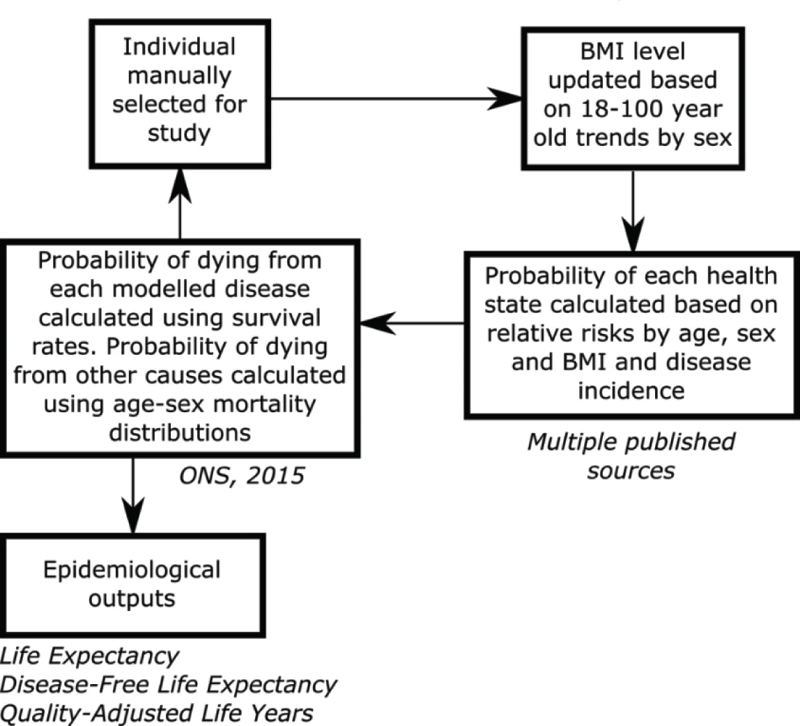
Figure 1 provides a summary of the main processes and data sources that were used in the individual-based model. An individual’s starting age, BMI and health status were pre-defined. Each year an individual’s BMI levels were updated based on the 18 to 100 year old BMI distribution trends disaggregated by sex. In this study the trends were assumed to be static, so the BMI distribution was assumed to be stationary, i.e. to not change over time. The 18 to 100 year old trends were computed by fitting a non-linear multivariate categorical regression model using individual level age, sex and BMI data from the 2013 Health Survey for England (HSE). The regression methods are described in the online supplementary material (Appendix). The model used an individual’s BMI, age and sex to calculate their risk of disease. The risk of disease was calculated from BMI-age-sex relative risks and age-sex incidence rates. Five obesity-related diseases were included in the simulation: coronary heart disease; stroke; type 2 diabetes; hypertension; and colorectal cancer. The individual-based model calculated the probability of each health state ranging from the probability of not having a disease to the probability of death. The probability of an individual living with multi-morbidities was also assessed up to a combination of four diseases at any one time. The probability of an individual dying was calculated from the survival rates of a given disease and the mortality rates of other causes (more technical details are provided in the online supplementary material ’ Appendix). The total mortality statistics and some of the survival statistics were sourced from the Office for National Statistics (ONS). In cases, where the survival statistics were unavailable the rates were estimated from prevalence and mortality statistics. Further details about these data sources are provided in the online supplementary material ’ Appendix. A utility weight was associated with each disease and these were used to estimate the mean Quality Adjusted Life Year (QALY) each year. The sources for this data are summarised in the online supplementary material ’ Appendix.

**Figure 1.** Schematic of the individual-based chronic disease model used to simulate individuals through time.

2.1.1 Case studies

Two 20-year-old case-studies were investigated: an overweight male (BMI=27.5 kg/m²) and an obese male (BMI=37.5 kg/m²). Both individuals had no health conditions in the start year of the simulation (2016). The model was simulated between 2016 and 2116 to ensure that the individuals are simulated far enough into the future to estimate life expectancy.

2.1.2 Model outputs

Obesity is a major risk factor for fatal (e.g. coronary heart disease) and non-fatal (e.g. type 2 diabetes) diseases and has been shown to have an impact on an individual’s healthy life expectancy (disease-free life expectancy) (Stenholm et al., 2017). Three outputs were assessed in this study: life expectancy, disease-free life expectancy and quality-adjusted life years. Life expectancy was calculated from the sum of the probabilities of the individual being alive in each year of the simulation and was initialised with the age of the individual in the start year of the simulation (see Equation 1). The disease-free life expectancy was calculated from the sum of the probability of an individual being alive without a disease in each year of the simulation (see Equation 2). This health metric was also initialised with the starting age of the individual. The quality-adjusted life year was initialised with the age of the individual in the start year of the simulation. It was calculated by summing the probability of being alive without a disease and the probability of being alive with a disease multiplied by the average quality of life (QoL) in the given year (see Equation 4). The average QoL was calculated from the utility weights which were specific to the diseases that an individual may have in a given year (see Equation 3). The average QoL was weighted based on the probability of having each disease.

(1)

Life expectancy = a g e (t_{s t a r t}) + \sum_{t = t_{s t a r t}}^{t_{e n d}} p_{a l i v e} (t)

(2)

Disease free life expectancy = a g e (t_{s t a r t}) + \sum_{t - t_{s t a r t}}^{t_{e n d}} (p_{a l i v e} (t) -_{p a l i v e + d i s e a s e} (t))

(3)

{QoL}_{a v e r a g e} (t) = \frac{\sum_{d = 0}^{N_{d i s e a s e s}} p_{d i s e a s e (t) \times {QoL}_{d i s e a s e}}}{\sum_{d = 0}^{N_{d i s e a s e}_{s}} p_{d i s e a s e} (t)}

(4)

Quality-adjusted life year = a g e (t_{s t a r t}) + \sum_{t = t_{s t a r t}}^{t_{e n d}} (p_{a l i v e + n o d i s e a s e} (t) + p a l i v e + d i s e a s e (t) \times {QoL}_{a v e r a g e} (t))

Equations 1, 2 and 4 are discrete time dynamic equations in steps of one year. The first term on the right hand side of these equations gives the age of the individual at the start of the simulation. The summation term of Equation 1 sums the probabilities that the individual is alive at each year. The summation term of Equation 2 only sums the probabilities that the individual is disease-free. The summation term of Equation 4 sums the probabilities that the individual is alive with no disease and the probabilities that the individual is alive with a disease scaled by the average QoL.

2.1.3 Model input parameter uncertainty

Information on the uncertainty from three different model input parameters was available in the literature and included in this analysis. The first model parameter was the BMI distribution trends. BMI trends by 5 year age groups were created for males, providing information on the probability of individuals in each BMI category (healthy weight, overweight and obese) across each 5 year age group from 2003 to 2116. The mean and standard deviation for each BMI category were calculated across all of the adult age groups (≥ 20 years old) between 2003 and 2116 (see Table 1). The overall mean probability and standard deviation across all of the BMI categories were also calculated from the mean and standard deviation from each BMI category. The upper and lower bounds for the healthy weight, overweight, obese and average BMI category probabilities were calculated by assuming a uniform distribution of uncertainty around each probability. Uniform distribution is often used as an uninformed prior distribution when there is a lack of precise information on parameter uncertainty. This provided an estimation of the uncertainty around the proportions of individuals within each BMI category.

In general, BMI distributions in a population are represented by a log-normal distribution. A log-normal distribution of the average adult male BMI levels was constructed from the mean probabilities of each BMI category. The mean BMI level (25.192) at the percentile corresponding to the mean BMI category probability (0.333) was estimated. In addition, the lower and upper bounds for the mean BMI level were estimated at the lower and upper bounds of the mean BMI category probability. The mean BMI level and the corresponding lower and upper bounds were used to estimate the lower and upper bounds around the BMI of each case study. It was assumed that the difference between the mean BMI level and the lower and upper bounds was the same as the difference between the BMI level of each case study and the corresponding lower and upper bounds (see Table 1).

Table 1. Summary of the BMI model parameters and their variances used in the sensitivity analysis.

Model parameter	Mean	Standard deviation	Lower bound	Upper bound
Healthy weight BMI probability (BMI < 25 kg/m²⁾	0.252	0.078	0.117	0.387
Overweight BMI probability (25 ≤ BMI < 30 kg/m²)	0.314	0.083	0.170	0.459
Obese BMI probability (BMI ≥ 30 kg/m²)	0.434	0.107	0.248	0.619
Mean BMI category probability	0.333	0.090	0.177	0.490
Mean BMI¹ level	25.192		20.591	27.028
Case study 1 BMI level	27.5		22.899	29.336
Case study 2 BMI level	37.5		35.207	41.644

The second and third parameters used in the uncertainty analysis were the relative risk of stroke and colorectal cancer, respectively. These were chosen because there were uncertainty estimates available in the literature. Granular relative risks were available by age and sex groups from the DYNAMO-HIA project (World Obesity Federation, 2008). An average of the overweight (25–30 kg/m²) and obese (≥ 30–45 kg/m²) groups was calculated for males. Variance estimates around each of these relative risks were not provided. The variance of the relative risk of stroke and colorectal cancer for overweight and obese were sourced from Guh et al. (2009) and used as a proxy for the variances around the DYNAMO-HIA relative risks. As this dataset contained only a single relative risk estimate for the overweight and obese categories, the estimates did not vary with age. The uncertainty was represented by a uniform distribution around each mean relative risk (see Table 2). The upper and lower bounds of each uniform distribution are presented in Table 2.

Table 2. Summary of the relative risk model parameters and their variances used in the sensitivity analysis.

Model parameter	Mean	Standard deviation	Lower bound	Upper bound
Relative risk stroke for overweight	1.213	0.056	1.116	1.310
Relative risk stroke for obese	1.758	0.107	1.573	1.944
Relative risk colorectal cancer overweight for	1.231	0.082	1.089	1.373
Relative risk colorectal cancer obese for	1.823	0.224	1.435	2.211

2.2 Sobol (Global) sensitivity indices

Denote the uncertain input parameters by x₁ … x_n where n is the number of uncertain parameters. The three uncertain input parameters used in this study represented the BMI value, relative risk of stroke and relative risk of colorectal cancer. Denote further by y the output (outcome) of interest and by f the analytical model or the black-box model (i.e. computer model) which maps the input parameters to the output (Equation 5):

(5)

y = f (x_{1}, x_{2}, ..., x_{n})

where the output parameter y represents life expectancy, disease-free life expectancy and quality-adjusted life years. The aim of the global sensitivity analysis method is to determine the contribution of the uncertainty (variance) in each of the input parameters x₁ … x_n (V_i(x_i)) and their interactions (V_ij(x_i,x_j)) to the uncertainty (variance) of the output y. The total number of parameters m of the model can of course be much larger than n, i.e. m » n. However, what is important here are the parameters which are considered to be uncertain. The variance of the output can be decomposed as follows (Equation 6):

(6)

V (f (x)) = \sum_{i = 1}^{n} V_{i} (x_{i}) + \sum_{1 \leq i < j \leq n} V_{i j} (x_{i}, x_{j}) + \sum_{1 \leq i < j < k \leq n} V i_{j k} ... + V_{1.... n}

Where V(f(x)) is the variance of the output, i.e. the variance of the life expectancy, disease-free life expectancy and quality-adjusted life year. This variance is composed of the variance from individual input model parameters (V_i(x_i)), variance from the interaction of two input model parameters (V_ij(x_i,x_j)) and the variance from the interaction of three or more input model parameters. In other words, the total variance of the output is the sum of the variances of the input parameters and all the orders of their interactions.

Sobol indices are a measure of global sensitivity analysis (Kucherenko, 2009; Saltelli, 2002; Saltelli et al., 2008, 2010; Sobol, 2001). They enable the quantification of the contribution of individual model input parameters and their interaction to the total variance of the model output parameter (V). The first order Sobol indices (S_i) relate to the individual contribution from each parameter (see Equation 7).

(7)

S_{i} = \frac{V_{i}}{V}

The second order Sobol indices relate to the interaction between two parameters i and j. The contribution from each pair of interactions is described in Equation 8.

(8)

S_{i j} = \frac{V_{i j}}{V}

Each Sobol index must be less than one and the sum of all the sensitivity indices is one (Equation 9).

(9)

\sum_{i}^{n} S_{i} + \sum_{i < j}^{n} S_{i j} + \sum_{i < j < k}^{n} S_{i j k} + ... = 1

The main assumption of the global sensitivity analysis method is that these parameters are independent. If required, the global sensitivity analysis method can be modified to handle dependence between the parameters by using Copulas (Kucherenko, Tarantola, & Annoni, 2012).

2.3 Analysing the Sobol indices for each model output

The first and second order Sobol indices for each model output were analysed with PSUADE, an open-source software package developed by Charles Tong (Tong, 2005). The software was used to generate auxiliary variables (z₁, z₂ and z₃) which were used as scalar additives to vary the true model input parameters within the uncertainty bounds. This was required because the relative risks for stroke and colorectal cancer varied with age and the uncertainty estimates for these model parameters were extracted from a source which only provided the uncertainty around single relative risks for all age groups. The uncertainties provided around these single relative risks were used as a proxy for the uncertainty around all the relative risks which varied with age and BMI. As an individual aged through the course of the simulation, they would be assigned a new probability of acquiring a disease based on their current age, sex and BMI. The distribution of each variable z₁, z₂ and z₃ sampled randomly with PSUADE in the start year of the simulation are summarised in Table 3. The variables z₁, z₂ and z₃ were used to scale the BMI, relative risk of stroke and relative risk of colorectal cancer, respectively in the model as shown in Equations 10 to 12.

Table 3. Scalar additives z₁, z₂ and z₃ sampled by PSUADE.

PSUADE parameter	Lower bound for overweight	Upper bound for overweight	Lower bound for obese	Upper bound for obese
z₁	22.899	29.336	35.207	41.644
z₂	1.116	1.310	1.573	1.944
z₃	1.089	1.373	1.435	2.211

(10)

B M I (t) = (z_{1} - B M I_{m e a n}) + B M I_{t r e n d} (t)

(11)

R R_{s t r o k e} (B M I, a g e) = (z_{2} - R R_{S t r o k e M e a n}) + R R_{s t r o k e} (B M I, a g e)

(12)

R R_{b o w e l} (B M I, a g e) = (z_{3} - R R C o l o r e c t a l C a n c e r M e a n) + R R C o l o r e c t a l C a n c e r (B M I, a g e)

The BMI prevalence and relative risk were correlated in the model because the relative risk was dependent on the BMI level. Constraints were applied on the parameters z₂ and z₃ which were scalar additives for the relative risks of stroke and colorectal cancer, respectively to account for this dependency. The relative risks for both diseases varied for two different age groups and by BMI. For each age group, a linear function was fitted to the relative risk by BMI level. For each disease, an average linear function was calculated from the linear functions approximated for the two age groups (further details are provided in online supplementary material). These average linear functions for stroke (see Equation 13) and colorectal cancer (see Equation 14) were used to define constraints on the sampled variables (z1, z₂ and z₃).

(13)

| z_{2} + 0.26095 - 0.0539 * z_{1} | < 0.1

(14)

| z_{3} + 0.36905 - 0.0585 * z_{1} | < 0.1

3. Results

In this section, the uncertainty analysis for life expectancy, disease-free life expectancy and quality-adjusted life year will be shown for both case studies: an overweight and an obese male aged 20 in 2016. The uncertainty for each of the model outputs will be shown in terms of the first-and second-order Sobol indices. For each model input parameter that has been studied, it will be checked if they are strictly positive and contribute to the uncertainty of each model output.

3.1 Disease-free life expectancy

The mean, standard deviation and variance of the disease-free life expectancy are summarised in Table 4. The mean number of year’s disease free was shown to be greater for the overweight male compared to the obese male 63 and 48 years, respectively. The standard deviation around the obese male mean disease-free life expectancy was similar to the standard deviation around the overweight disease-free life expectancy mean.

Table 4. Summary of the mean, standard deviation and variance for the disease-free life expectancy for the two case studies.

Case study	Mean (years)	Standard deviation (years)	Variance (years²)
Overweight male	63.47	3.41	11.59
Obese male	48.32	3.14	9.87

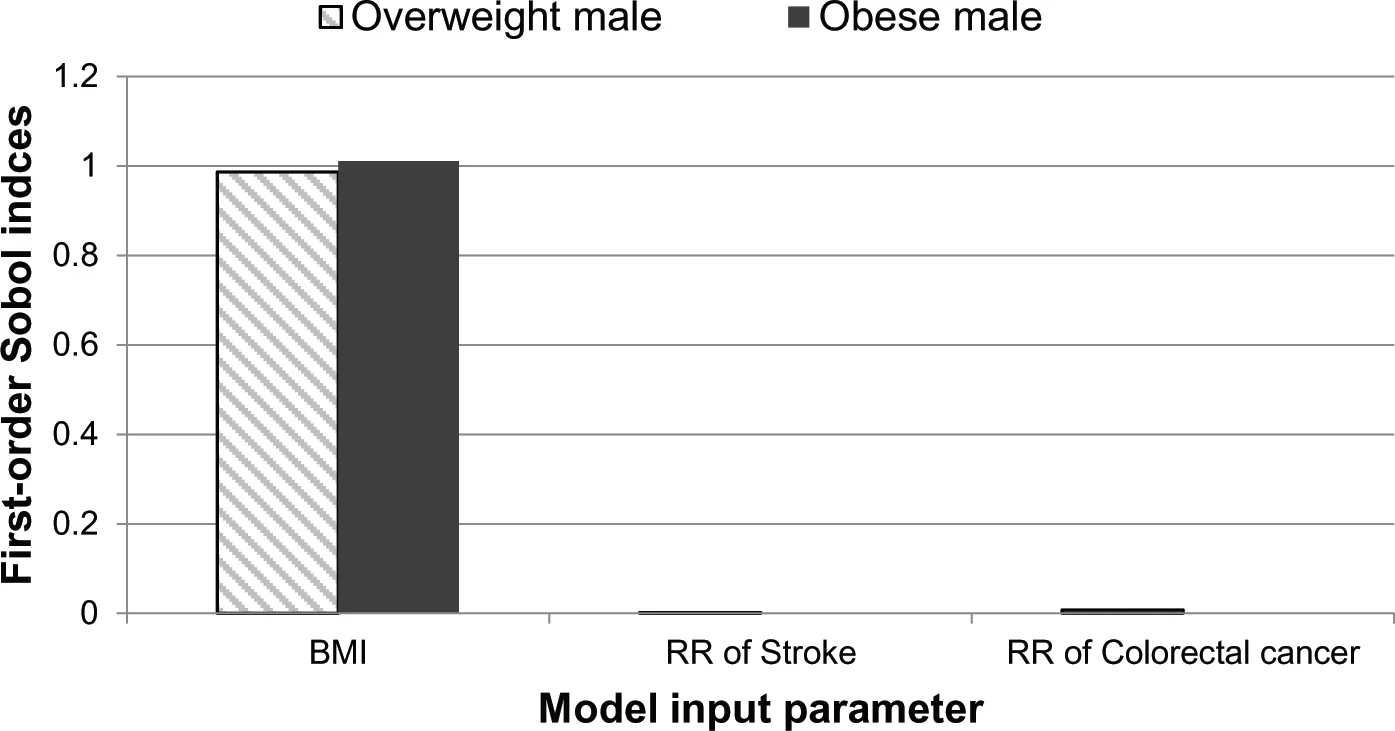
The individual impact of the uncertainty of the three input parameters on the disease-free life expectancy is shown in Figure 2. The graph shows the first-order Sobol indices for each of the three input parameters. The first parameter, which relates to the BMI value, is shown to have the greatest impact on the overall uncertainty of the disease-free life expectancy output for both the overweight and obese males. The smallest impact is from the parametric uncertainty of the relative risk of stroke for both case studies. For the overweight male, there was shown to be a much larger difference between the BMI and relative risk first-order Sobol indices.

**Figure 2.** A graphical illustration of the first-order Sobol indices for each model input parameter: BMI, relative risk of stroke and relative risk of colorectal cancer for disease-free life expectancy.

The second-order Sobol indices were not strictly positive and did not contribute to the uncertainty of the disease-free life expectancy.

3.2 Life expectancy

The impact of the parametric uncertainty of the three model input parameters on the life expectancy was much smaller compared to the disease-free life expectancy. Table 5 shows the mean, standard deviation and variance life expectancy for each case study.

Table 5. Summary of the mean, standard deviation and variance for the life expectancy for the two case studies.

Case study	Mean (years)	Standard deviation (years)	Variance (years²)
Overweight male	79.76	0.11	0.01
Obese male	79.17	0.31	0.09

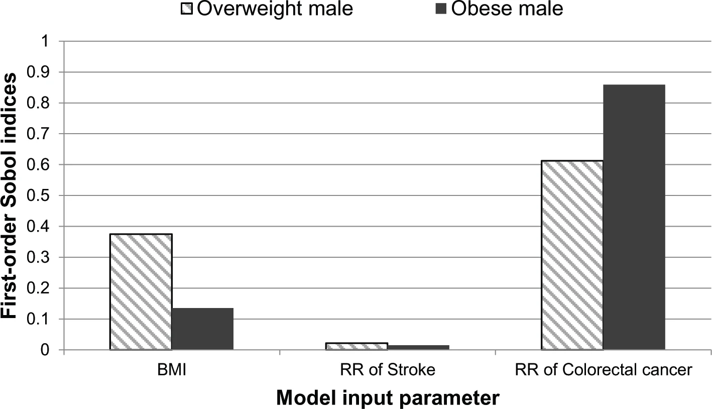
There was a mean life expectancy difference of approximately 0.6 years between the overweight and obese individuals. The standard deviations for the overweight and obese individuals were 0.11 and 0.31 years, respectively. The first-order Sobol indices were analysed for both case studies and the results are presented in Figure 3. The results show that the uncertainty from the relative risk of colorectal cancer contributes the most to the overall uncertainty of the life expectancy. However, the BMI also contributes to the uncertainty.

**Figure 3.** A graphical illustration of the first-order Sobol indices for each model input parameter: BMI, relative risk of stroke and relative risk of colorectal cancer for life expectancy.

The second-order Sobol indices were not strictly positive and did not contribute to the uncertainty of the life expectancy.

3.2 Quality-adjusted life years

The mean quality-adjusted life years for an overweight and an obese male were 75 and 70 years, respectively (Table 6). The standard deviations around each of the case studies were similar.

Table 6.

Case study	Mean (years)	Standard deviation (years)	Variance (years²)
Overweight male	75.09	1.01	1.02
Obese male	70.06	1.06	1.12

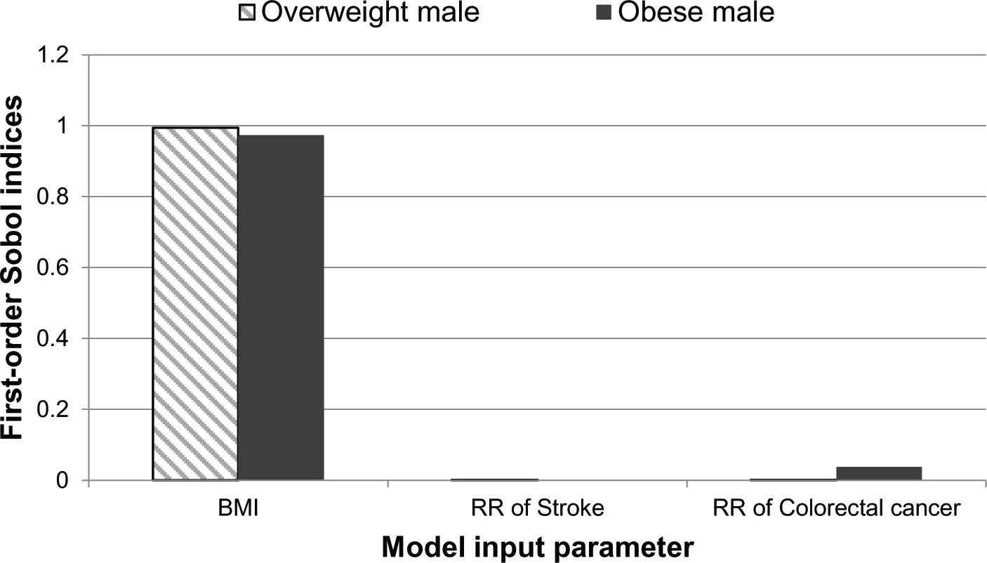
The impact from each of the model parameters is shown in Figure 4. The relative impact from each of the three model parameters on the uncertainty of the quality-adjusted life year outputs were similar to the results observed for disease-free life expectancy. BMI has the greatest contribution to the overall uncertainty of the quality adjusted life years for both the overweight and obese case studies. In the overweight case study, BMI is the only model parameter which contributes to the quality-adjusted life year uncertainty when compared to the relative risk of stroke and relative risk of colorectal cancer. For the obese male both BMI and the relative risk of colorectal cancer have an impact on the uncertainty of this model output.

**Figure 4.** A graphical illustration of the first-order Sobol indices for each model input parameter: BMI, relative risk of stroke and relative risk of colorectal cancer for quality-adjusted life year.

The second-order Sobol indices were not strictly positive and did not contribute to the uncertainty of the quality adjusted life year.

4. Discussion

We have estimated the uncertainty of three model outputs: life expectancy, disease-free life expectancy and quality-adjusted life years in an individual based model. Global sensitivity analysis was carried out to calculate the contribution from BMI trends, relative risk of stroke and relative risk of colorectal cancer on the uncertainty of the life expectancy, disease-free life expectancy and quality-adjusted life years. An overweight and an obese male were modelled as case studies. BMI is shown to have an impact on the mean disease-free life expectancy and quality-adjusted life years and only a small impact on mean life expectancy. From the three input parameters investigated only the uncertainty from the BMI trends contributed to the uncertainty of the disease-free life expectancy and the uncertainty of the quality adjusted life year for the overweight case study. However, the life expectancy uncertainty was influenced by the BMI trends and relative risk of colorectal cancer uncertainties. To our knowledge, this is the first time that global sensitivity analysis has been applied to an individual-based chronic disease model (Hennessy et al., 2015; Lymer et al., 2016; Manuel et al., 2014).

4.1 Disease-free life expectancy

An individual’s disease-free life expectancy was calculated by the summing over the annual probabilities that an individual lived without a disease in their lifetime. The model simulated additional obesity-related diseases which were not included in the global sensitivity analysis. The uncertainties for these parameters were not included because the uncertainty estimates around these model input parameters were difficult to reliably source. These model parameters included the relative risks of type 2 diabetes, hypertension and coronary heart disease. The probability that an individual acquired a disease was primarily driven by BMI. The uncertainty of the relative risk of stroke and colorectal cancer did not have an effect on the incidence of type 2 diabetes, hypertension and coronary heart disease. The uncertainty of the BMI trends was therefore likely to have a larger influence on the disease-free life expectancy uncertainty.

A large difference in the mean disease-free life expectancy was observed between an overweight and an obese male. This was expected because obese individuals have a greater probability of acquiring obesity related diseases. The uncertainty of the disease-free life expectancy for the obese male was relatively larger than the overweight male disease-free life expectancy. This is related to there being a greater uncertainty around the model input parameters for the obese male.

4.2 Life expectancy

The contribution from the model input parameters to the uncertainty of life expectancy was more distributed amongst the model inputs for the overweight and obese male. The uncertainty of the life expectancy estimate was much smaller compared to the uncertainty of the disease-free life expectancy. The model also takes account of deaths from other causes. The uncertainty of the mortality rates from other causes was not incorporated into this uncertainty analysis. Therefore, uncertainty reported in this study is likely to underestimate the total uncertainty. The BMI trends are likely to have had a smaller effect on life expectancy compared to disease-free life expectancy because of the type of additional diseases that were modelled in this study. Type 2 diabetes and hypertension were non terminal diseases, which would not impact on the life expectancy. As previously discussed these diseases did have an impact on disease-free life expectancy. Moreover, each case study had vastly different BMI levels, 27.5 kg/m² and 37.5 kg/m² and only a small difference was observed in the mean life expectancy. This evidence suggests that the uncertainty in BMI levels would only have a small impact on the life expectancy uncertainty. The uncertainty of the relative risk of colorectal cancer also contributed to the uncertainty of life expectancy compared to the relative risk of stroke. The uncertainties around relative risks for colorectal cancer were greater than the uncertainties for the stroke relative risks. Therefore, the colorectal cancer relative risk uncertainties were more likely to contribute to the life expectancy uncertainties compared to the stroke relative risks.

4.3 Quality-adjusted life year

The total quality-adjusted life years for an individual were calculated based on the probability that an individual had a particular disease and the probability that an individual was disease free. The probability that an individual had a particular disease was scaled by the QoL of the individual in a given year. The average QoL was estimated from the diseases that an individual may have in a given year. The QoL for an individual varies between zero (dead) and one (alive and disease-free). The quality-adjusted life year for an obese individual was lower compared to the overweight individual. This is because an obese individual is more likely to be living with obesity related diseases. It is unlikely that the probability of death had an impact on this difference in the quality-adjusted life years between the overweight and obese individual because there were only very small differences between the mean life expectancies of the two case studies.

BMI was the only model parameter to contribute to the uncertainty of quality-adjusted life year for the overweight case study. A similar outcome was observed for the disease-free life expectancy. BMI and the relative risk of colorectal cancer contributed to the uncertainty of the quality adjusted life years for the obese individual. Colorectal cancer had a QoL equal to 0.68 compared to stroke which had a QoL equal to 0.713. The diseases that have a lower QoL are likely to have a larger impact on the quality-adjusted life years. In addition, the obese individual had a higher chance of acquiring colorectal cancer compared to the overweight individual. Therefore, it was more likely that the uncertainty of the colorectal cancer relative risks would have a larger impact on the uncertainty of this model output for the obese individual. Additional diseases were included in the simulation but not in the uncertainty analysis. Diseases such as type 2 diabetes also have a relatively low QoL equal to 0.66. It is highly likely that the uncertainty of the relative risks for type 2 diabetes would also have an influence on the uncertainty of the quality-adjusted life years if they were included in the uncertainty analysis.

4.4 Limitations

There are limitations in this study with regards to the sources of uncertainty, the assumptions used to approximate the uncertainty and the small subset of parameters assessed. One limitation relates to the estimation of the uncertainty from the BMI trends. The average uncertainty was obtained from averaging the uncertainty across each five year age group and BMI category and up to 100 years into the future. However, the uncertainty in the BMI projections did not remain constant and actually increased over time. The uncertainty of the BMI used in this analysis is likely to be an overestimate. Further work will investigate whether a time varying uncertainty can be included in the global sensitivity analysis. This is particularly important because the time horizon of interest will vary depending on the starting age of an individual. Future work will need to adapt the uncertainty estimation based on the time horizon of interest. Another limitation relates to the sample size used by the PSUADE program. This was set to 20,000 samples. However, after the samples were filtered based on the constraints, the sample size was reduced to 31% and 12% of the original samples for the overweight and obese case studies, respectively. In order to scale this process to the microsimulation, an optimal number of samples required will need to be assessed to minimise the computational time taken to run the model.

We were unable to obtain uncertainty estimates for all of the parameters used in the model. A high number of model input parameters were sourced from published literature (see the online supplementary material for further details). In many cases the uncertainties of these point estimates were not provided. In this study it was only possible to obtain the standard deviations around one overweight and one obese relative risk for stroke and colorectal cancer (Guh et al., 2009). The uncertainties were not disaggregated by age or sex. However, a different source was used to approximate the mean point estimates for the model (World Obesity Federation, 2008). Overweight and obese case studies were chosen based on the uncertainty data available for relative risks. These data were more granular and were broken down by age, sex and BMI groups. More granular data was preferred for the individual based model, as the relative risks varied between different age, sex and BMI groups. The standard deviations obtained from the less granular relative risks were used as a proxy for the granular relative risks. These uncertainties may have been overestimated because age, sex and BMI may have contributed to the uncertainty around the less granular relative risks. In general, the risk of these diseases increases with age. Therefore, the uncertainty used when the individual was in their 20’s to 40’s may have overestimated the uncertainty from these parameters. Although, when an individual reached an older age, this uncertainty may have been underestimated. This will depend on the original cohort used to estimate the relative risks and their associated uncertainties.

We have addressed only parametric uncertainty in this study. We did not address structural uncertainty. By their nature, model parameters are, however, conditional on model structure. Structural uncertainty is concerned with the uncertainty in the structure of the model. This can take several forms such as the uncertainty in the high-level methodological assumptions made to construct the model (e.g. in relation to characterising the health trajectory of an individual), the uncertainty in the number of state variables in the model (e.g. number of disease and health states), the uncertainty in the relationships governing the associations between the model variables (e.g. the associations between disease relative risk and BMI and age). There are various methods to address structural uncertainty but we have not incorporated any of them in this study (Bojke, Claxton, Sculpher, & Palmer, 2009; Strong, Oakley, & Chilcott, 2012).

This study has focused on a method for assessing parametric uncertainty in complex nonlinear models. This is important for models where the outputs are used by decision makers and therefore need to be trusted. Modelling standards for good research practices have been developed by the International Society for Pharmacoeconomics and Outcomes Research to improve the reliability and transparency of models reported in the literature (Caro, Briggs, Siebert, & Kuntz, 2012). These good research practices highlight the need to include uncertainty analysis in addition to validation and comparisons with other models in the field. Internal and external validation is an important and consistent theme across a number of modelling guidelines (American Diabetes Association Consensus Panel, 2004; Caro et al., 2012; Palmer et al., 2013). The uncertainty analysis method described in this study will contribute towards standardising dissemination of modelling outputs.

4.5 Future work

This study has focused on a small subset of model input parameters to demonstrate the application of applying global sensitivity analysis techniques to an individual based model, a simplified version of the UK Health Forum (UKHF) microsimulation model. This study is a precursor for applying global sensitivity analysis to the UKHF microsimulation model. Future work will increase the number of model input parameters that are incorporated into the global sensitivity analysis. In addition, the method will be scaled up in order to incorporate differences from within a population in the microsimulation model. However, future analyses will optimise this process by identifying the key model input parameters that contribute to the uncertainty of different model outputs and assess the sample and population sizes required to obtain accurate uncertainty estimates which can help inform public health policies.

Footnotes

1.

The average BMI was approximated from the BMI distribution in 2013 as predicted by the static trend. The BMI was calculated from the average BMI category percentile mean, lower and upper bounds.

Appendix

A. Technical appendix for the individual based model

An individual j at age a, in year y has a risk factor (RF) value rf_j (a,y) (e.g. BMI). The set of RF values for all possible integer ages is termed a RF trajectory {rf (a₀, y₀), rf (a₀ + 1, y₀ + 1),.., rf (a_max, y₀ + a_max −a₀)}. In this model, the RF trajectories are assumed to be static, so an individual’s BMI value will not change over time. At any age, a person will be in one of many exclusive and exhaustive states. The state update equation (Equation A1) is

(A1)

p_{s i} (a + 1, y + 1, s) = \sum_{j = 0}^{j = | s | - 1} T_{i j} (a, y, s) p_{S j} (a, y, s)

where, T is the state-transition matrix and |S| are the total number of states. The set of states is complete so that, for all a, and s, for each year y, the probabilities of state membership are (Equation A2)

(A2)

\sum_{i = 0}^{i = | s | - 1} p_{S i} (a, y, s) = 1

where p_Si (a, y, s) is the probability of being in state i at age a in year y with sex s. The possible health states range from alive with no disease, alive with a disease and dead. An individual can have a maximum of four different diseases at any one time. The probability that an individual acquires a disease d is calculated from the calibrated incidence p_Id (a, y₀, s|rf₀) and relative risk (RR) $ρ_{R F j}^{d} (a, s)$ of the disease given the individual’s BMI value. In Equation A3 the disease incidence probabilities are given as

(A3)

p_{I d} = p_{I d} (a, y_{0}, s | r f_{j}) = ρ_{r f_{j}}^{d} (a, s) p_{I d} (a, y_{0}, s | r f_{0})

where the RR $ρ_{R F j}^{d} (a, s)$ is that appropriate to the RF group rf_j, which is the group identified by the element rf (a, y, s) of the person’s RF trajectory. This is assumed to hold for subsequent years.

The input disease incidence data are used to determine the probabilities of disease incidence for a zero-risk (RF group 0, rf₀) person — the probability p_Id (a, y₀|rf₀). This is calculated as (Equation A4)

(A4)

p_{I d} (a_{0}, y_{0}, s | r f_{0}) = \frac{{\bar{p}}_{I d} (a_{0}, y_{0}, s)}{\sum_{j = 0}^{j = | R F | - 1} ρ_{R F j} (a_{0}, s) p_{R F j} (a_{0}, y_{0}, s)}

where, the probability of being in a RF group p_RFj(a₀, y₀, s) is determined from the 5 year age and sex group trends.

Each year an individual may die from a disease or from other causes. The probability that an individual dies from other causes is calculated from the total mortality rates by age and sex. These rates are available from the Office for National Statistics (ONS). The probability that an individual dies from a specific disease is calculated from the survival probabilities. If an individual has multiple disease their probability of dying is calculated as shown in Equation (A5).

(A5)

\begin{array}{l} p_{ω 1} = p_{Ω 0} (1 - p_{Ω 1}) + p_{Ω 1} (1 - p_{Ω 0}) \\ p_{ω 2} = p_{Ω 0} (1 - p_{Ω 2}) + p_{Ω 2} (1 - p_{Ω 0}) \\ p_{ω 12} = p_{Ω 0} (1 - p_{Ω 1}) (1 - p_{Ω 2}) + p_{Ω 1} (1 - p_{Ω 2}) (1 - p_{Ω 0}) + p_{Ω 2} (1 - p_{Ω 0}) (1 - p_{Ω 1}) \end{array}

B. Estimating the relationship between relative risks of colorectal cancer and stroke by body mass index

The RR for colorectal cancer and stroke were estimated from the DYNAMO-HIA project (World Obesity Federation, 2008). An equation was provided for both RRs, which described how the RR could be approximated for each BMI value for two different age groups. For each disease, the RR was plotted against the BMI value for the two different age groups (Figures B.1 and B.2). A linear equation was fitted to each age group for each disease.

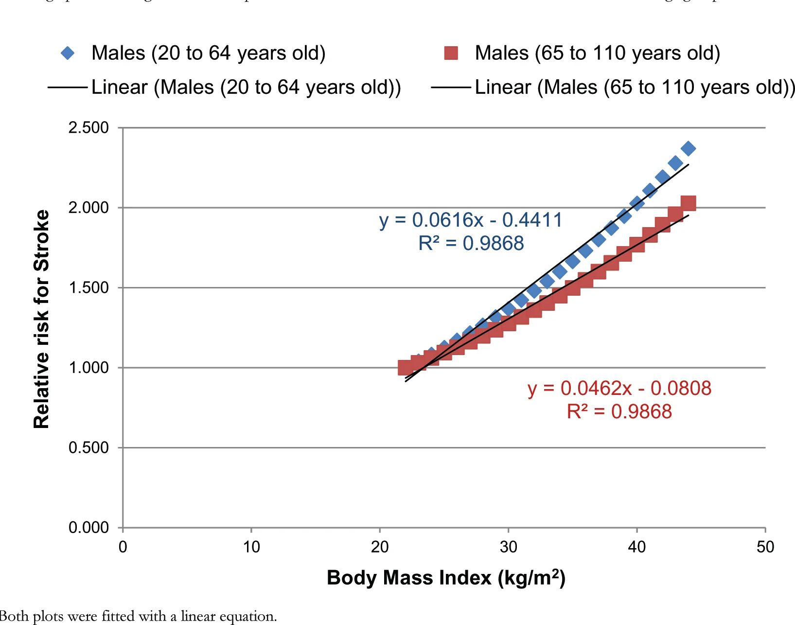
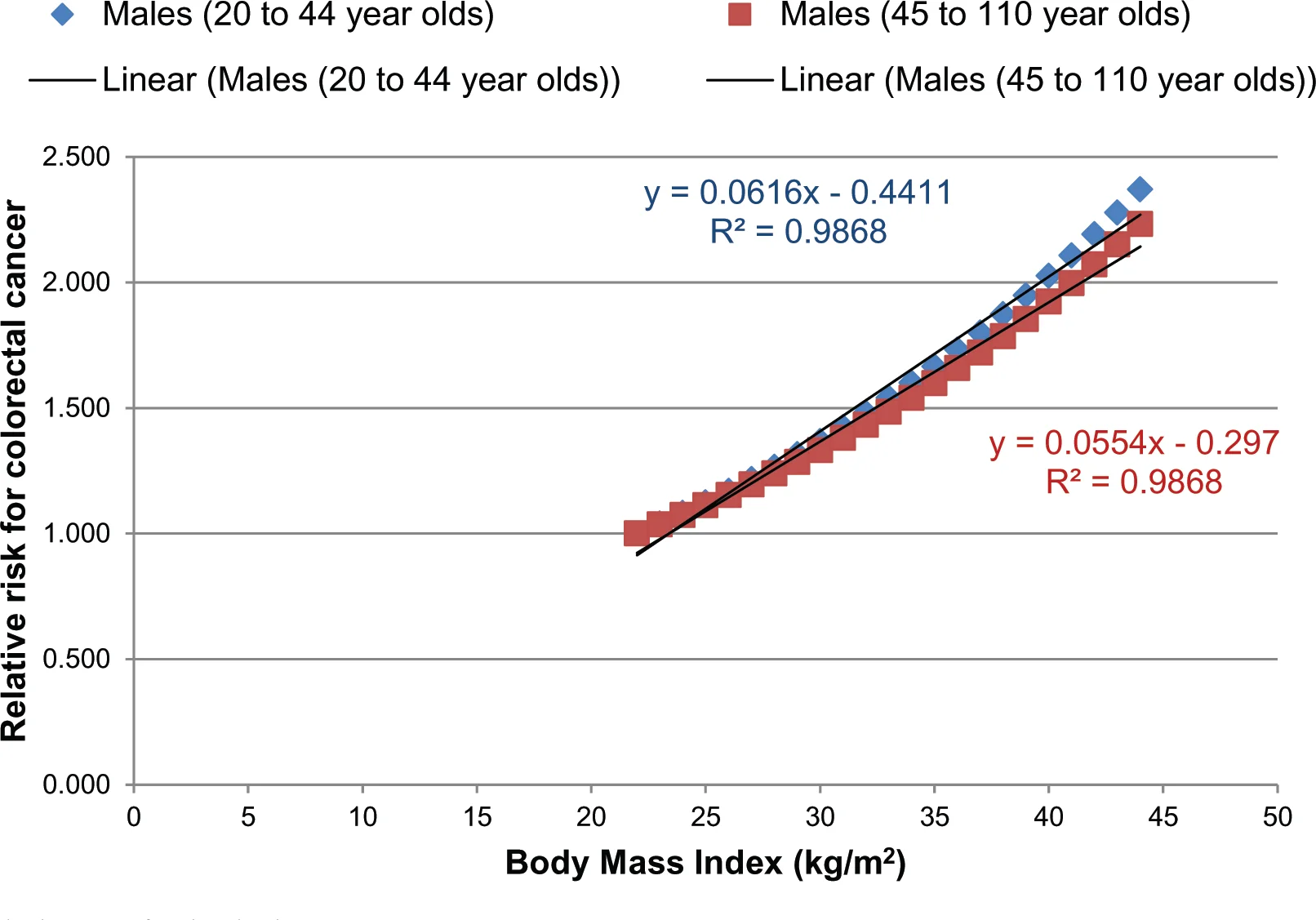
**Figure B.1.** A graph illustrating the relationship between the RR for stroke and BMI for males for two different age groups.

**Figure B.2.** A graph illustrating the relationship between the RR for colorectal cancer and BMI for males for two different age groups.

A mean RR was calculated for the overweight (25–30 kg/m²) and obese (30–45 kg/m²) groups for each age group and each disease. A uniform distribution was assumed for each mean. The upper and lower bounds were calculated from the mean using the standard deviation from Guh et al. (2009).

Due to the dependency of BMI on the RR constraints were used within PSUADE. These constraints were calculated by taking the average of the two linear functions for each age group for each disease.

C. Computing BMI trends

BMI is analysed within the model as a RF, as described in Table C.1.

Table C.1. Description of the categories used for the RF BMI.

Risk factor (RF)	Number of categories (N)	Categories
BMI	3	BMI < 25 kg/m² (normal weight)
		BMI from 25 to 29.99 kg/m^-2 (overweight)
		BMI ≥ 30 kg/m² (obesity)

For the RF, let N be the number of categories for a given RF, e.g. N = 3 for BMI. Let k = 1, 2, …, N number these categories and p_k(t) denote the prevalence of individuals with RF values that correspond to the category k at time t. We estimate p_k(t) using multinomial logistic regression model with prevalence of RF category k as the outcome, and time t as a single explanatory variable. For k < N, we have (Equation C1)

(C1)

\ln (\frac{p_{k} (t)}{p_{1} (t)}) = β_{0}^{k} + β_{0}^{k} t

The prevalence of the first category is obtained by using the normalisation constraint $\sum_{k = 1}^{N} p_{k} (t) = 1$ . Solving Equation C2 for p_k(t), we obtain

(C2)

p_{k} (t) = \frac{\exp (β_{0}^{k} + β_{1}^{k} t)}{1 + \sum_{k' = 1}^{N} \exp (β_{0}^{k'} + β_{1}^{k'} t)},

which respects all constraints on the prevalence values, i.e. normalisation and [0, 1] bounds.

C.1 Multinomial logistic regression for risk factor BMI

Measured data consist of sets of probabilities, with their variances, at specific time values (typically the year of the survey). For any particular time, the sum of these probabilities is unity. Typically, such data might be the probabilities of normal weight, overweight and obese as they are extracted from the survey data set. Each data point is treated as a normally distributed random variable; together they are a set of N groups (number of years) of K probabilities {{t_i, µ_ki, σ_ki|k∈[0,K-1]} | i∈[0,N-1]}. For each year, the set of K probabilities form a distribution — their sum is equal to unity.

The regression consists of fitting a set of logistic functions {p_k(a, b, t)|k∈[0,K-1]} to these data — one function for each k-value. At each time value, the sum of these functions is unity. Thus, for example, when measuring obesity in the three states already mentioned, the k = 0 regression function represents the probability of being normal weight over time, k = 1 the probability of being overweight, and k = 2 the probability of being obese.

The regression equations are most easily derived from a familiar least square minimization. In the following equation set (Equations C3 and C4) the weighted difference between the measured and predicted probabilities is written as S and the logistic regression functions p_k(a,b;t) are chosen to be ratios of sums of exponentials. This is equivalent to modelling the log probability ratios, p_k/p₀, as linear functions of time.

(C3)

S (a, b) = \frac{1}{2} \sum_{k = 0}^{k = K - 1} \sum_{i = 0}^{i = N - 1} \frac{{(p_{k} (a, b; t_{i}) - μ_{k i})}^{2}}{σ_{k i}^{2}}

(C4)

\begin{array}{l} p_{k} (a, b;t) = \frac{e^{A_{k}}}{1 + e^{A_{1}} + .. + e^{A_{K - 1}}} \\ a \equiv (a_{0}, a_{1}, .., a_{K - 1}), b \equiv (b_{0}, b_{1}, .., b_{K - 1}) \\ A_{0} \equiv 0, ​ ​ A_{k} \equiv a_{k} + b_{k} t \end{array}

The parameters A₀, a₀ and b₀ are all zero and are used merely to preserve the symmetry of the expressions and their manipulation. For a K-dimensional set of probabilities, there will be 2(K-1) regression parameters to be determined. For a given dimension K there are K-1 independent functions p_k — the remaining function being determined from the requirement that complete set of K form a distribution and sum to unity.

Note that the parameterization ensures that the necessary requirement that each p_k be interpretable as a probability is a real number lying between 0 and 1. The minimum of the function S is determined from the Equations C5. and C6:

(C5)

\frac{\partial S}{\partial a_{j}} = \frac{\partial S}{\partial b_{j}} = 0 for j=1,2, ....,k-1

noting the relations

(C6)

\begin{array}{l} \frac{\partial p_{k}}{\partial A_{j}} = \frac{\partial}{\partial A_{j}} (\frac{e^{A_{k}}}{1 + e^{A_{1}} + .. + e^{A_{K - 1}}}) = p_{k} δ_{k j} - p_{k} p_{j} \\ \frac{\partial}{\partial a_{j}} = \frac{\partial}{\partial A_{j}} \\ \frac{\partial}{\partial b_{j}} = t \frac{\partial}{\partial A_{j}} \end{array}

The values of the vectors a, b that satisfy these equations are denoted $\hat{a}, \hat{b}$ . They provide the trend lines $p_{k} (\hat{a}, \hat{b}; t)$ , for the separate probabilities. The confidence intervals for the trend lines are derived most easily from the underlying Bayesian analysis of the problem.

C.2 Bayesian interpretation

The 2K-2 regression parameters {a,b} are regarded as random variables whose posterior distribution is proportional to the function exp(-S(a,b)). The maximum likelihood estimate of this probability distribution function, the minimum of the function S, is obtained at the values $\hat{a}, \hat{b}$ . Other properties of the (2K-2)-dimensional probability distribution function are obtained by first approximating it as a (2K-2)-dimensional normal distribution whose mean is the maximum likelihood estimate. This amounts to expanding the function S(a,b) in a Taylor series as far as terms quadratic in the differences $(a - \hat{a}), (b - \hat{b})$ about the maximum likelihood estimate $\hat{S} \equiv S (\hat{a}, \hat{b})$ . Hence the Equation C7 is written as follows:

(C7)

\begin{array}{l} S (a, b) = \frac{1}{2} \sum_{k = 0}^{k = K - 1} \sum_{i = 0}^{i = N - 1} \frac{{(p_{k} (a, b; t_{i}) - μ_{k i})}^{2}}{σ_{k i}^{2}} \\ \equiv S (\hat{a}, \hat{b}) + \frac{1}{2} (a - \hat{a}, b - \hat{b}) P^{- 1} (a - \hat{a}, b - \hat{b}) + ... \\ \approx S (\hat{a}, \hat{b}) + \frac{1}{2} \sum_{i, j} (a_{i} - {\hat{a}}_{i}) \frac{\partial^{2} \hat{S}}{\partial {\hat{a}}_{i} \partial {\hat{a}}_{j}} (a_{j} - {\hat{a}}_{j}) + \frac{1}{2} \sum_{i, j} (a - {\hat{a}}_{i}) \frac{\partial^{2} \hat{S}}{\partial {\hat{a}}_{i} \partial {\hat{b}}_{j}} (b_{j} - {\hat{b}}_{j}) + \\ + \frac{1}{2} \sum_{i, j} (b_{i} - {\hat{b}}_{j}) \frac{\partial^{2} \hat{S}}{\partial {\hat{b}}_{i} \partial {\hat{a}}_{j}} (a_{j} - {\hat{a}}_{j}) + \frac{1}{2} \sum_{i, j} (b_{i} - {\hat{b}}_{i}) \frac{\partial^{2} \hat{S}}{\partial {\hat{b}}_{i} \partial {\hat{b}}_{j}} (b_{j} - {\hat{b}}_{j}) \end{array}

The (2K-2)-dimensional covariance matrix P is the inverse of the appropriate expansion coefficients. This matrix is central to the construction of the confidence limits for the trend lines.

C.3 Estimation of the confidence intervals

The logistic regression functions p_k(t) can be approximated as a normally distributed time-varying random variable $N ({\hat{p}}_{k} (t), σ_{k}^{2} (t))$ by expanding p_k about its maximum likelihood estimate (the trend line) ${\hat{p}}_{k} (t) = p (\hat{a}, \hat{b}, t)$ (Equation C8).

(C8)

\begin{array}{l} p_{k} (a, b, t) = p_{k} (\hat{a} + a - \hat{a}, \hat{b} + b - \hat{b}, t) \\ = {\hat{p}}_{k} (t) + (\nabla_{\hat{a}}, \nabla_{\hat{b}}) {\hat{p}}_{k} (t) (\begin{matrix} \begin{matrix} a - \hat{a} \\ b - \hat{b} \end{matrix} \end{matrix}) + ... \end{array}

Denoting mean values by angled brackets, the variance of p_k is thereby approximated as (Equation C9):

(C9)

\begin{array}{l} σ_{k}^{2} (t) \equiv 〈 {(p_{k} (a, b, t) - {\hat{p}}_{k} (t))}^{2} 〉 = (\nabla_{\hat{a}} {\hat{p}}_{k} (t)) 〈 (\begin{matrix} a - \hat{a} \\ b - \hat{b} \end{matrix}) {(\begin{matrix} a - \hat{a} \\ b - \hat{b} \end{matrix})}^{T} 〉 \times \\ {(\nabla_{\hat{a}} {\hat{p}}_{k} (t), \nabla_{\hat{b}} {\hat{p}}_{k} (t))}^{T} = (\nabla_{\hat{a}} {\hat{p}}_{k} (t), \nabla_{\hat{b}} {\hat{p}}_{k} (t)) P {(\nabla_{\hat{a}} {\hat{p}}_{k} (t), \nabla_{\hat{b}} {\hat{p}}_{k} (t))}^{T} \end{array}

When K=3 this equation can be written as the 4-dimensional inner product (Equation C10):

(C10)

σ_{k}^{2} (t) = (\frac{\partial {\hat{p}}_{k} (t)}{\partial {\hat{a}}_{1}} \frac{\partial {\hat{p}}_{k} (t)}{\partial {\hat{a}}_{2}} \frac{\partial {\hat{p}}_{k} (t)}{\partial {\hat{b}}_{1}} \frac{\partial {\hat{p}}_{k} (t)}{\partial {\hat{b}}_{2}}) [\begin{matrix} P_{a a 11} & P_{a a 12} & P_{a b 11} & P_{a b 12} \\ P_{a a 21} & P_{a a 22} & P_{a b 21} & P_{a b 22} \\ P_{b a 11} & P_{b a 12} & P_{b b 11} & P_{b b 12} \\ P_{b a 21} & P_{b a 22} & P_{b b 21} & P_{b b 22} \end{matrix}] (\begin{matrix} \frac{\partial {\hat{p}}_{k} (t)}{\partial {\hat{a}}_{1}} \\ \frac{\partial {\hat{p}}_{k} (t)}{\partial {\hat{a}}_{2}} \\ \frac{\partial {\hat{p}}_{k} (t)}{\partial {\hat{b}}_{1}} \\ \frac{\partial {\hat{p}}_{k} (t)}{\partial {\hat{b}}_{2}} \end{matrix})

where $P_{c d i j} \equiv 〈 (c_{i} - {\hat{c}}_{i}) (d_{j} - {\hat{d}}_{j}) 〉$ . The 95% confidence interval for p_k(t) is centred given as $[{\hat{p}}_{k} (t) - 1.96 σ_{k} (t), p_{k} (t) + 1.96 σ_{k} (t)]$ .

Disease	Incidence	Prevalence	Mortality	Survival	Relative Risk	Utility Weight
CHD	Smolina et al 2012. Corrected data on incidence and mortality in 2013 (Smolina, Wright, Rayner, & Goldacre, 2012)	BHF, Cardiovascular Disease Statistics 2014 (British Heart Foundation, 2015)	ONS, Deaths Registrations Summary Statistics, England and Wales, 2014 (Office for National Statistics, 2014)	Computed from prevalence and mortality	World Obesity Federation (DYNAMO project) (World Obesity Federation)	Laires et al. 2015 (Laires, Ejzykowicz, Hsu, Ambegaonkar, & Davies, 2015)
Stroke	BHF, stroke statistics 2009 (British Heart Foundation, 2009)	BHF, Cardiovascular Disease Statistics 2014 (British Heart Foundation, 2015)	ONS, Deaths Registrations Summary Statistics, England and Wales, 2014 (Office for National Statistics, 2014)	Computed from prevalence and mortality	World Obesity Federation (DYNAMO project) (World Obesity Federation)	Rivero-Arias et al. 2010 (Rivero-Arias et al., 2010)
Hypertension	Derived from prevalence	Health Survey for England 2012 (Health and Social Care Information Centre, 2012)	non terminal	non terminal	World Obesity Federation (DYNAMO project) (World Obesity Federation)	Sullivan et al. 2011 (Sullivan, Slejko, Sculpher, & Ghushchyan, 2011)
Diabetes	Personal communication Dr. Craig Currie at Cardiff University	National Diabetes Audit 2015–2016(NHS Digital, 2017)	non terminal	non terminal	World Obesity Federation (DYNAMO project) (World Obesity Federation)	Sullivan et al. 2011 (Sullivan et al., 2011)
Colorectal cancer	CRUK, 2013 Statistics by cancer type (Cancer Research UK, 2016b)	NA	CRUK Mortality by cancer type(Cancer Research UK, 2016a)	ONS Cancer Survival in England: adults diagnosed between 2009 and 2013 and followed up to 2014 (Office for National Statistics, 2015) & ONS Cancer Survival in England: 10 year survival rates adults diagnosed between 2010–2011 and followed up to 2012 (Office for National Statistics, 2013)	World Obesity Federation (DYNAMO project) (World Obesity Federation)	Sullivan et al. 2011 (Sullivan et al., 2011)

References

Ahern, AL, Wheeler, GM, Aveyard, P, Boyland, EJ, Halford, JC, Mander, AP, Cole, D (2017). Extended and standard duration weight-loss programme referrals for adults in primary care (WRAP): a randomised controlled trial. The Lancet, 389, 2214–2225.
(2004). Guidelines for computer modeling of diabetes and its complications. Diabetes Care, 27, 2262–2265.
Atella, V, Belotti, F, Carrino, L, Piano Mortari, A (2017). The future of Long Term Care in Europe. An investigation using a dynamic microsimulation model.
Bojke, L, Claxton, K, Sculpher, M, Palmer, S (2009). Characterizing structural uncertainty in decision analytic models: a review and application of methods. Value in Health, 12, 739–749.
Caro, JJ, Briggs, AH, Siebert, U, Kuntz, KM (2012). Modeling good research practices— overview: a report of the ISPOR-SMDM Modeling Good Research Practices Task Force–1. Medical decision making, 32, 667–677.
Goldman, DP, Zheng, Y, Girosi, F, Michaud, PC, Olshansky, SJ, Cutler, D, Rowe, JW (2009). The benefits of risk factor prevention in Americans aged 51 years and older. American journal of public health, 99, 2096–2101.
Gonzalez-Gonzalez, C, Tysinger, B, Goldman, DP, Wong, R (2017). Projecting diabetes prevalence among Mexicans aged 50 years and older: the Future Elderly Model-Mexico (FEM-Mexico). BMJ open, 7.
Guh, DP, Zhang, W, Bansback, N, Amarsi, Z, Birmingham, CL, Anis, AH (2009). The incidence of co-morbidities related to obesity and overweight: a systematic review and meta-analysis. BMC public health, 9.
Hennessy, DA, Flanagan, WM, Tanuseputro, P, Bennett, C, Tuna, M, Kopec, J, Manuel, DG (2015). The Population Health Model (POHEM): an overview of rationale, methods and applications. Population health metrics, 13.
Hunt, D, Knuchel-Takano, A, Jaccard, A, Bhimjiyani, A, Retat, L, Selvarajah, C, Brown, M (2017). Modelling the implications of reducing smoking prevalence: the public health and economic benefits of achieving a ‘tobacco-free’UK. Tobacco Control, 2016–053507.
Kucherenko, S (2009). Derivative based global sensitivity measures and their link with global sensitivity indices. Mathematics and computers in simulation, 79, 3009–3017.
Kucherenko, S, Tarantola, S, Annoni, P (2012). Estimation of global sensitivity indices for models with dependent variables. Computer Physics Communications, 183, 937–946.
Kypridemos, C, Allen, K, Hickey, GL, Guzman-Castillo, M, Bandosz, P, Buchan, I, O’Flaherty, M (2016). Cardiovascular screening to reduce the burden from cardiovascular disease: microsimulation study to quantify policy options. BMJ, 353.
Lymer, S, Schofield, D, Lee, CM, Colagiuri, S (2016). NCDMod: A Microsimulation Model Projecting Chronic Disease and Risk Factors for Australian Adults. International Journal of Microsimulation, 9, 103–139.
Manuel, DG, Tuna, M, Hennessy, D, Bennett, C, Okhmatovskaia, A, Finès, P, Team, STfAR (2014). Projections of preventable risks for cardiovascular disease in Canada to 2021: a microsimulation modelling approach. CMAJ open, 2.
Mathijssen, J, Petersen, A, Besseling, P, Rahman, A, Don, H (2008). Dealing with Uncertainty in Policymaking. Netherlands Environmental Assessment Agency, Netherlands Bureau for Economic Policy Analysis and Rand Europe.
McPherson, K, Marsh, T, Brown, M (2007). Tackling obesities: future choices: Modelling future trends in obesity and the impact on health. Department of Innovation, Universities and Skills.
Palmer, AJ, , Clarke, P, Gray, A, Leal, J, Lloyd, A, Valentine, W (2013). Computer modeling of diabetes and its complications: a report on the Fifth Mount Hood challenge meeting. Value in Health, 16, 670–685.
Rogers, SM, Rineer, J, Scruggs, MD, Wheaton, WD, Cooley, PC, Roberts, DJ, Wagener, DK (2014). A geospatial dynamic microsimulation model for household population projections. International Journal of Microsimulation, 7, 119–146.
Rutter, CM, Zaslavsky, AM, Feuer, EJ (2011). Dynamic microsimulation models for health outcomes: a review. Medical decision making, 31, 10–18.
Saltelli, A (1999). Sensitivity analysis: Could better methods be used?. Journal of Geophysical Research: Atmospheres, 104, 3789–3793.
Saltelli, A (2002). Making best use of model evaluations to compute sensitivity indices. Computer Physics Communications, 145, 280–297.
Saltelli, A, Annoni, P, Azzini, I, Campolongo, F, Ratto, M, Tarantola, S (2010). Variance based sensitivity analysis of model output. Design and estimator for the total sensitivity index. Computer Physics Communications, 181, 259–270.
Saltelli, A, Ratto, M, Andres, T, Campolongo, F, Cariboni, J, Gatelli, D, Tarantola, S (2008). Global sensitivity analysis: the primer. John Wiley & Sons.
Sharif, B, Kopec, JA, Wong, H, Finès, P, Sayre, EC, Liu, RR, Wolfson, MC (2012). Uncertainty analysis in population-based disease microsimulation models.
Sobol, IM (2001). Global sensitivity indices for nonlinear mathematical models and their Monte Carlo estimates. Mathematics and computers in simulation, 55, 271–280.
Stenholm, S, Head, J, Aalto, V, Kivimäki, M, Kawachi, I, Zins, M, Hanson, LM (2017). Body mass index as a predictor of healthy and disease-free life expectancy between ages 50 and 75: a multicohort study. International journal of obesity (2005), 41.
Strong, M, Oakley, JE, Chilcott, J (2012). Managing structural uncertainty in health economic decision models: a discrepancy approach. Journal of the Royal Statistical Society: Series C (Applied Statistics), 61, 25–45.
Tong, C (2005). Psuade user’s manual. Livermore, CA: Lawrence Livermore National Laboratory (LLNL).
(2008). https://s3.eu-central-1.amazonaws.com/ps-wof-web-dev/site_media/uploads/Appendix_Relative_Risk_Assessments_IASO.pdf. https://s3.eu-central-1.amazonaws.com/ps-wof-web-dev/site_media/uploads/Appendix_Relative_Risk_Assessments_IASO.pdf.
(2016). Statistics by cancer type – Average Number of Deaths per Year and Age-Specific Mortality Rates, UK, 2010-2012. http://www.cancerresearchuk.org/health-professional/cancer-statistics/statistics-by-cancer-type.
(2016). Statistics by cancer type – Average Number of New Cases Per Year and Age-Specific Incidence Rates per 100,000 Population, UK 2011-2013. http://www.cancerresearchuk.org/health-professional/cancer-statistics/statistics-by-cancer-type.
Guh, DP, Zhang, W, Bansback, N, Amarsi, Z, Birmingham, CL, Anis, AH (2009). The incidence of co-morbidities related to obesity and overweight: a systematic review and meta-analysis. BMC Public Health, 9.
(2012). https://digital.nhs.uk/data-and-information/publications/statistical/health-survey-for-england/health-survey-for-england-2012. https://digital.nhs.uk/data-and-information/publications/statistical/health-survey-for-england/health-survey-for-england-2012.
Laires, PA, Ejzykowicz, F, Hsu, TY, Ambegaonkar, B, Davies, G (2015). Cost– effectiveness of adding ezetimibe to atorvastatin vs switching to rosuvastatin therapy in Portugal. Journal of Medical Economics, 18, 565–572.
(2017). http://www.content.digital.nhs.uk/catalogue/PUB23241. http://www.content.digital.nhs.uk/catalogue/PUB23241.
(2013). Cancer Survival in England: 10 year survival rates adults diagnosed between 2010-2011 and followed up to 2012. https://www.ons.gov.uk/peoplepopulationandcommunity/healthandsocialcare/conditions anddiseases/bulletins/cancersurvivalinenglandadultsdiagnosed/2010and2014andfollowedu pto2015.
(2014). Deaths Registrations Summary Statistics, England and Wales. https://www.ons.gov.uk/peoplepopulationandcommunity/birthsdeathsandmarriages/deat hs/datasets/deathregistrationssummarytablesenglandandwalesreferencetables.
(2015). Cancer Survival in England-Adults Diagnosed: 2009 to 2013, followed up to 2014. https://www.ons.gov.uk/peoplepopulationandcommunity/healthandsocialcare/conditions anddiseases/bulletins/cancersurvivalinenglandadultsdiagnosed/2009to2013followedupto20 14.
Rivero-Arias, O, Ouellet, M, Gray, A, Wolstenholme, J, Rothwell, PM, Luengo-Fernandez, R (2010). Mapping the modified Rankin scale (mRS) measurement into the generic EuroQol (EQ-5D) health outcome. Medical Decision Making, 30, 341–354.
Scarborough, P, Peto, V, Bhatnagar, P, Kaur, A, Leal, J, Luengo-Fernandez, R, Allender, S (1000). Stroke Statistics 2009 edition. British Heart Foundation Statistics Database.
Smolina, K, Wright, FL, Rayner, M, Goldacre, MJ (2012). Determinants of the decline in mortality from acute myocardial infarction in England between 2002 and 2010: linked national database study.
Sullivan, PW, Slejko, JF, Sculpher, MJ, Ghushchyan, V (2011). Catalogue of EQ-5D scores for the United Kingdom. Medical Decision Making.
Townsend, N, Williams, J, Bhatnagar, P, Wickramasinghe, K, Rayner, M (1000). Cardiovascular Disease statistics 2014. British Heart Foundation.
(1000). Relative risk Assessments IASO; Prepared for DYNAMO-HIA project. http://www.worldobesity.org/site_media/uploads/Appendix_Relative_Risk_Assessments_IASO.pdf.
(2008). Relative Risk assessments: Prepared for the Dynamo-HIA project. https://s3.eu-central-1.amazonaws.com/ps-wof-web-dev/site_media/uploads/Appendix_Relative_Risk_Assessments_IASO.pdf.

Article and author information

Author details

Abbygail Jaccard
UK Health Forum, United Kingdom
For correspondence: Abbygail.Jaccard@gmail.com
Lise Retat
UK Health Forum, United Kingdom
For correspondence: Lise.Retat@ukhealthforum.org.uk
Martin Brown
UK Health Forum, United Kingdom
For correspondence: mbcltd@btinternet.com
Laura Webber
UK Health Forum, United Kingdom
For correspondence: Laura.Webber@ukhealthforum.org.uk
Zaid Chalabi
Department of Public Health, Environments and Society, London School of Hygiene and Tropical Medicine, United Kingdom
For correspondence: Zaid.Chalabi@lshtm.ac.uk

Acknowledgements

The research is partially funded by the UK Health Forum and partially funded by the National Institute for Health Research Health Protection Research Unit (NIHR HPRU) in Environmental Change and Health at the London School of Hygiene and Tropical Medicine in partnership with Public Health England (PHE), and in collaboration with the University of Exeter, University College London, and the Met Office. The views expressed are those of the author(s) and not necessarily those of the NHS, the NIHR, the Department of Health or Public Health England. We are thankful to Dr Charles Tong for his valuable expertise in using the PSUADE programme, which greatly assisted this analysis.

Publication history

Version of Record published: December 31, 2018 (version 1)

Copyright

This article is distributed under the terms of the Creative Commons Attribution License, which permits unrestricted use and redistribution provided that the original author and source are credited.