
Jump to
1. Introduction
Sociodemographic microsimulation can be used to model and understand the development of populations, their behaviors, and outcomes. Microsimulations play an increasingly important role in modeling the complex dynamics of public health phenomena as well as in the investigation of causal mechanisms and intervention effects (Jackson and Arah, 2020; Lee et al., 2019; Monteiro et al., 2016; Stephen and Barnett, 2017). Synthetic populations are datasets that have been reweighted to represent geographical areas that can represent populations at the individual level (Tanton, 2014). This approach allows for the investigation of behaviors and outcomes at an individual-level and breakdowns by demographic categories, and also allows for the updating of populations over time, i.e. using mortality or migration rates (Ballas et al., 2007).
An estimated 72,558 annual deaths in the USA can be attributed to alcohol use, with liver disease and alcohol overdose or poisoning accounting for 30.7% and 17.9% of these deaths, respectively (White et al., 2020). Indeed globally, alcohol is a major cause of the burden of disease (Griswold et al., 2018). Alcohol use in the US varies substantially by age, gender and socio-demographics, (Delker et al., 2016) and the National Survey on Drug Use and Health (NSDUH) provides a detailed individual level dataset with which to examine these patterns. In 2018, 24.5% of the population aged 12+ were estimated to drink 5+ standard drinks (technically 14g of pure ethanol, which is roughly equivalent to a 12 fluid ounce can of 5% strength beer) during the previous month Substance Abuse and Mental Health Services Administration (2019).
Our context here is a US National Institute on Alcohol Abuse and Alcoholism funded project called “Calibrated Agent Simulations for Combined Analysis of Drinking Etiologies (CASCADE)”. CASCADE aims to: (1) develop new computer models of alcohol use which draw on existing theories for why people drink and seek novel combinations of these theories in order to better explain the changes in alcohol use we observe in society; (2) provide policymakers with insight into how alcohol-related harms, particularly alcohol poisoning and liver disease, have developed over the last 35 years; (3) guide development of new policies by providing projections for how levels of harm might change under different future intervention scenarios. The microsimulation model we present in this paper forms part of a wider software architecture for modelling social systems, for more details see (Vu et al., 2020b). Our model is intended to provide a demographically representative population over time, which can be used for individual-level and agent-based simulation models and supports the adding of mechanisms to generate individual level behavior.
Several microsimulation studies around alcohol exist, and have studied aspects of treatment for alcohol dependence using microsimulation (Millier et al., 2017). Others have used microsimulation to analyse screening and brief interventions for alcohol problems (Zur and Zaric, 2016). (Brennan et al., 2015; Holmes et al., 2014) have developed a hybrid modelling approach with part individual, part cohort level analysis of alcohol use and resulting harms for alcohol policy analysis. However, to date there is not large scale, long term (30+ years) microsimulation of populations and their alcohol use.
Some sociodemographic microsimulations already exist. In the US, we reviewed the Framework for Reconstructing Epidemic Dynamics (FRED) microsimulation for infectious diseases (Grefenstette et al., 2013) which developed a synthetic population based on the US Census Bureau’s Public Use Microdata Sample and aggregated data from the 2005-2009 American Community Survey (ACS) (Wheaton et al., 2009). The FRED microsimulation provided insights on methods/data sources. In particular, we require that simulated individuals have characteristics that are representative of known features of the population e.g. the proportion of males and females, age distribution, and proportion employed/unemployed are representative. The standard approach to ensuring a simulated dataset fits these representativeness criteria is iterative proportional fitting (IPF) (Lovelace et al., 2015; Lovelace and Dumont, 2016). However, the micro-synthetic population and microsimulation implemented in FRED has a number of limitations. Firstly, they cover only a short timeframe (2005-2009), which is not far enough historically to explain long-run public health. Secondly, they are static and do not account for core demographic developments such as births, deaths, and migration. Thirdly, the model focusses on communicable diseases and does not include risk factors, such as alcohol, for non-communicable diseases.
The objective of our study was to develop a more comprehensive sociodemographic micro-synthesis and microsimulation - CASCADEPOP version 1.0, assess its validity on sociodemographic outputs and provide transparent open-source code for the research community.
2. Methods
2.1. CASCADEPOP requirements
CASCADEPOP was required to develop a simulated set of individuals with US state representative sociodemographic characteristics, starting on 01/01/1980 and to simulate individuals’ characteristics and baseline health behaviors (e.g. alcohol use) over time to 31/12/2015, also allowing for births, migrations, and deaths. This 35-year timeframe allows investigation of long-term changes e.g., in total alcohol per capita consumption, decreasing gender differences in alcohol use, and recent decreases in young people’s alcohol use (Keyes et al., 2008; Martinez et al., 2019; Patrick and Schulenberg, 2014).
CASCADEPOP has been developed for any US state and here we operationalize micro-synthesis and microsimulation for five states, California (CA), Minnesota (MN), New York (NY), Tennessee (TN), Texas (TX) and the US. These states were chosen because they reflect heterogeneous patterns of population dynamics (different age and sex distributions, socioeconomics, race/ethnicity composition, and extent of migration over time) and because they have substantially different levels and trends in aggregate population per capita sales litres of alcohol (Martinez et al., 2019).
We focus on ages 12 through 80, though the methods can be utilized for other age categories. The sociodemographic characteristics implemented in the micro-synthesis were: Sex (male, female), age (continuous), race/ethnicity (non-Hispanic white, non-Hispanic black, Hispanic, other), level of education (high school or less, some college, college degree or higher), household annual income (8 groups: $0-6999, $7-$9,999, $10-14,999 $15-19,999, $20-24,999, $25-29,999, $30-34,999, $35,000+) employment status (employed, unemployed), marital status (married, unmarried), and parental status (no children living at home, at least one child aged below 18 living at home). These characteristics were considered key requirements for CASCADEPOP, because they are related to alcohol use and to many other health behaviors (Rehm et al., 2009; 2010; 2014). The microsimulation also needed to allow dynamic changes in sociodemographic characteristics as each individual progresses through his/her life while also being representative of the US population.
Our exemplar health behavior of alcohol use was implemented as follows. We categorize ‘drinking status’ into current drinkers and abstainers. We track average grams of alcohol per day consumed, frequency of drinking and of ‘heavy episodic drinking’ for each drinker, defined below.
2.2. Data sources
Generating a micro-synthetic base population and implementing dynamic changes in the population over time required the integration of a series of data sources described below.
2.2.1. US Census data
US Census data for 1980 were obtained from the National Geographic Information service (Manson et al., 2019) and used to inform sociodemographic characteristics of the base population in terms of the joint distribution of age (12-17, 18-24, 25-29, 30-34, 35-39, 40-44, 45-49, 50-59, 60-80), sex, race/ethnicity, marital status, employment status, level of education, and income. Census data for years 1990, 2000, and 2010 were used to inform the addition of new individuals entering the microsimulation at age 12 (instead of at birth).
2.2.2. Panel Study of Income Dynamics
The Panel Study of Income Dynamics (PSID) is a large, nationally representative US longitudinal survey, designed to measure the dynamics of income, wealth, and expenditures (University of Michigan. Survey Research Center, 2018). PSID was available annually from 1968-1997, and biennially from 1997-2015. The 1979 survey contains the required variables including sex, age (continuous), race/ethnicity, level of education, income, employment status, marital status, and parental status. Census data contain information on household composition but do not provide individual-level parental status. Therefore, we used 1980 PSID data to inform the distribution of parental status in the micro-synthesis, and used the longitudinal data to estimate social role transition probabilities (see Statistical Procedures).
2.2.3. American Community Surveys
Data from the American Community Survey (ACS) in 1980, 1990 and for individual years for 2000-2015 were used to inform immigration and emigration at state and national levels (Ruggles et al., 2019). ACS is a sub-sample (1%) of households in the US Census and contains individual-level demographic information (age, sex, race/ethnicity) and details on whether an individual has migrated in the previous five years (1980, 1990, 2000) or one year (2000-2015).
2.2.4. Compressed Mortality Files
Mortality rates before age 80 were based on the National Center for Health Statistics National Death Index database. Mortality rates were extracted using data from the Center for Disease Control and Prevention online databases for 1979-1998 (Centers for Disease Control and Prevention, National Center for Health Statistics. Compressed Mortality File, 1979) and 1999-2017 (Centers for Disease Control and Prevention, National Center for Health Statistics. Underlying Cause of Death, 1999). These provide a record of total deaths (from all causes) per year, aggregated by state, by age category, and sex.
2.2.5. National Survey on Drug Use and Health
To inform alcohol use behavior in the micro-synthetic population, we required an individual-level dataset containing sociodemographic variables alongside information on each individual’s pattern of alcohol use. For version 1.0 of CASCADEPOP, we selected the National Survey on Drug Use and Health (NSDUH) (U.S. Department of Health and Human Services, Substance Abuse and Mental Health Services Administration, Center for Behavioral Health Statistics and Quality, 2019).
NSDUH was selected because it provides individual-level nationally representative repeated cross-sections. NSDUH includes individuals aged 12+ across the US (excluding Alaska and Hawaii) based on a national area probability sample. NSDUH data were available for consecutive years 1979-2016 (excluding 1980-1981, 1983-1984 and 1989). The survey contains age in individual years (1979-1999) and in narrow category bands (1999-2016). Information on sex, race/ethnicity, level of education, income (in eight bands in earlier years, and as a continuous $ amount in later years), employment status, marital status, and parental status, are available in all survey years. For constructing the baseline population, income was expressed in 1980 U.S. dollars to correspond to the Census data. For the microsimulation, incomes for all years were converted 2015 dollars (US Bureau of Labor Statistics: Consumer Price Index. Washington, 2019).
NSDUH contains information on four alcohol use variables. ‘Drinking status’ is a binary variable defined as having used alcohol at least once in the past 12 months. Average grams per day of alcohol consumed was calculated based on the number of drinking days in the past 30 days and the number of drinks usually consumed per occasion (standard drink = 14 grams of alcohol e.g. a regular 12-ounce bottle of beer). Alcohol consumption frequency is the number of days where alcohol was consumed in the past 30 days (continuous). Frequency of ‘heavy episodic drinking’ is defined as the number of days in the past 30 days when over 5 standard drinks were consumed.
2.3. Statistical procedures
2.3.1. Iterative proportional fitting for 1980 population micro-synthesis
Iterative proportional fitting is a procedure that is used to reweight individual level data to fit the known demographic constraints of populations (Lovelace and Dumont, 2016). Further information about data preparation for iterative proportional fitting is available in Appendix A and B. The goal of the micro-synthesis was to provide a synthetic base population of individuals for the selected geography. For example, to generate the base CA population on 01/01/1980 of N=18,957,712, the aim was to generate a database with over 18 million records with the sociodemographic structure that matches the demographic constraints in the Census. The method to achieve this is IPF. IPF uses an iterative algorithm to estimate the cell values of a contingency table such that the marginal totals, known as IPF constraints, remain fixed.
For CASCADEPOP v1.0, incorporated constraints from different datasets (details in Appendix A and B). The process began with the individual-level dataset (NSDUH, 2019) which contained the drinking and sociodemographic variables described above. The sample size, after removing people who have missing required attributes, is n=6,105. The ipfp package (Blocker, 2016) was used to calculate a weight for each individual in the NSDUH, 2019 dataset so that the re-weighted NSDUH had a sociodemographic structure that fits the constraints of the geography of interest (done separately for CA, MN, NY, TN, TX, and the US) (See Appendix tables B3–B5).
The constraints used for IPF were (i) a three-way cross-tabulated combination of age categories, sex, and race/ethnicity, together with cross-tabulations of (ii) employment by sex, (iii) marital status by sex, (iv) level of education by sex, and (v) income categories by sex. The data for these constraints came from the US Census 1980 and the PSID 1980 datasets. In total, we used 138 constraints: 104 constraints for 13 age categories * 2 sex * 4 race/ethnicity categories 4 for marital status * sex, 4 for employment status * sex, 16 for income categories * sex, and 6 for education * sex.
The IPF algorithm used the 138-constraint vector and the individual characteristics of the NSDUH (N=6,105 rows in our case) to estimate a weight for each NSDUH individual so that the total number of individuals in each of the 138 constraint categories matched the constraints. The algorithm followed an iterative process until a tolerance level for the error (L2 norm Euclidean distance between the vector of the reweighted population number and the constraint vector) was reached (10-10). The final set of weights indicated the number of people each NSDUH individual represented in each geography. A replication process was then undertaken to generate a database with the correct total population of CA in 1980 (N=18,957,712) and all of the required fields (Lovelace and Ballas, 2013).
2.3.2. Iterative proportional fitting for immigration and new 12-year-olds over time
Migration and births mean that additional individuals enter the microsimulation in each year 1981 to 2015 (details in Appendix C).
To account for new 12-year olds, data from the US Census in 1990 for people aged 12-22 (who would have been aged 12 in 1980-1990) were used to generate constraints for individuals entering the model aged 12 in 1980-1990. Similarly, the 2000 Census was used to generate constraints for 1990-2000 and Census 2010 was used for constraints for 2000-2010 and 2011-2015.
To account for migration, ACS data were used to generate constraints for the net number of migrants to enter into each state and year (see details in Appendix C). ACS person weights were used to determine the number of individuals in the Census represented by each ACS individual, and ensure that these constraints were representative at a population level. For each state (CA, MN, NY, TN, TX), emigration (migration out of the state) was calculated using a weighted ACS to determine the age, sex, race/ethnicity, and year of migration of all individuals who emigrated from the state of interest to another state. We also accounted for new migrants between April and December in 1980 because the US Census date was 01/04/1980.
An IPF process, similar to that for the base 1980 population, was implemented separately for each state for each year from 1981 to 2010. The process began with the NSDUH dataset for the relevant year. For some years there was no NSDUH survey and we utilized the survey from the closest year. A vector of 104 constraints was used for migrants entering the geography (13 age categories * 2 sex * 4 race/ethnicity), and 8 constraints were used for new 12-year-olds entering the population (2 sex * 4 race/ethnicity). In most years, for most states, net immigration was positive i.e., more people entered than left the state. In the case where net migration was negative, we did not require an IPF process, but instead, we quantified net emigration by age, sex, and race/ethnicity and used Monte Carlo sampling to simulate people who left (see microsimulation section).
2.3.3. Estimating social role transitions over time
Multi-state Markov models describe and estimate how an individual moves through a series of states over time, and are commonly used for estimating transitions between stages of disease (Jackson et al., 2003). We defined eight social role combinations of marital status, parental status, and employment. Using longitudinal PSID data, we applied a time homogenous Multi-State Markov Model using the msm package in R (Jackson, 2007) to calculate age- and sex-dependent annual probabilities of transitioning in and out of each social role combination. Details of the number of single transitions between social roles available in PSID data are available in Appendix D. Separate models were estimated for five time periods (1979-1983, 1984-1992, 1993-1999, 2000-2007, 2008-2015). We included sex as a dichotomous covariate and age and age squared as continuous time-variant covariates. To illustrate, we show below the transition matrix for 1993-1999, for 27-year-old females (Table 1). Here, we see that if an individual in this category holds no social roles during this period, they are likely to still hold no social roles in 1 year (P=0.649), the most likely transition for an individual with no roles is to become employed (P=0.280), The full model transition intensities with hazard ratios for age and sex are available in Appendix Table D2.
| _ _ _ | _ _ P | _ M _ | E _ _ | _ M P | E M _ | E _ P | E M P | ||
|---|---|---|---|---|---|---|---|---|---|
| 1993-1999 | _ _ _ | 0.649 | 0.025 | 0.017 | 0.280 | 0.003 | 0.014 | 0.010 | 0.001 |
| 1993-1999 | _ _ P | 0.013 | 0.605 | <0.001 | 0.008 | 0.054 | <0.001 | 0.298 | 0.021 |
| 1993-1999 | _ M _ | 0.025 | 0.001 | 0.537 | 0.012 | 0.118 | 0.261 | 0.001 | 0.045 |
| 1993-1999 | E _ _ | 0.087 | 0.003 | 0.004 | 0.816 | 0.001 | 0.059 | 0.026 | 0.005 |
| 1993-1999 | _ M P | <0.001 | 0.010 | 0.005 | <0.001 | 0.677 | 0.003 | 0.007 | 0.297 |
| 1993-1999 | E M _ | 0.004 | <0.001 | 0.079 | 0.035 | 0.013 | 0.757 | 0.002 | 0.110 |
| 1993-1999 | E _ P | 0.003 | 0.091 | <0.001 | 0.030 | 0.006 | 0.001 | 0.817 | 0.051 |
| 1993-1999 | E M P | <0.001 | 0.002 | 0.001 | 0.001 | 0.083 | 0.013 | 0.025 | 0.876 |
The time-periods and covariates were selected due to annual data availability in the PSID, to ensure enough data was available to fit each model. These transition probabilities were applied during the microsimulation over time to simulate individuals transitioning between social roles each year.
2.4. Microsimulation over time
2.4.1. Socio-demographic microsimulation
Figure 1 provides an overview of the steps that happen to generate the baseline and migrant populations, and in each simulated year, with more details in Appendix E. The microsimulation proceeds on year by year basis. During each year, steps were implemented to account for aging, social role transitions, new 12-year-olds, deaths and migration. On January 1st of the next modelled year, each simulated person increases in age by +1 years. The probability that a simulated person moves from a particular combination of social roles e.g., married, employed, and a parent to another of the eight combinations was based on the transition matrices described above, operationalized using Monte Carlo sampling. New migrants and 12-year-olds enter the model for each year of the simulation. In the case of net emigration, we removed the estimated count of migrants to leave the state by age, sex and race/ethnicity category using Monte Carlo sampling. Individuals can also leave the simulation due to death – implemented by taking the total count of deaths by age category and sex and removing the corresponding number of individuals from the simulation, again using Monte Carlo sampling. Migration rates are adjusted according to a procedure described in detail in Appendix E to ensure correspondence with counts of the total population of each geography in 1990, 2000 and 2010. In the results presented here, we have tested the microsimulation at 10% scale due to computational constraints and all results are presented at this scale.
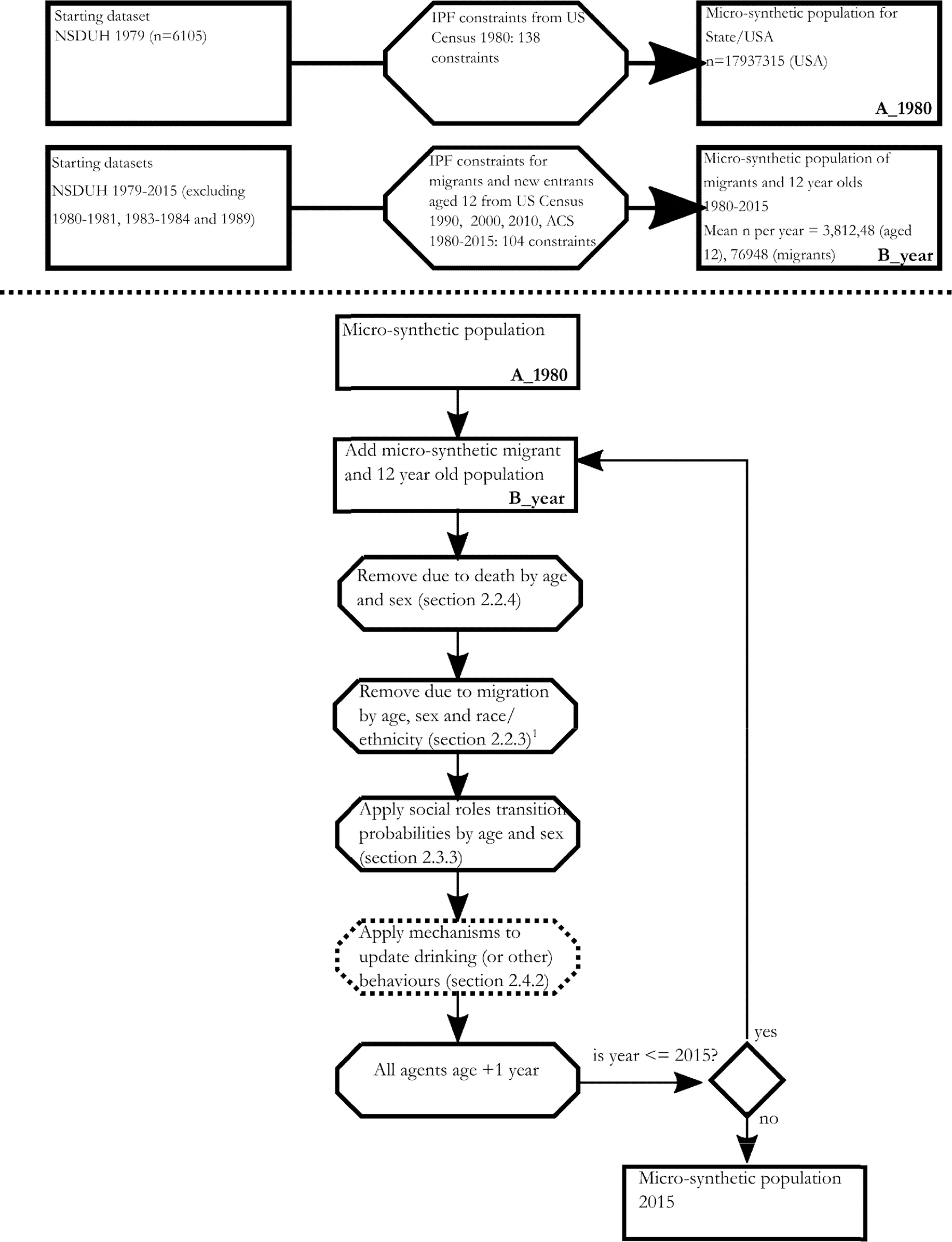
2.4.2. Place within the structure for incorporating mechanisms into the microsimulation
The dynamic microsimulation also enables the updating of the individual drinking behavior (and other behavior – if required) over time. These are not discussed in depth in this paper, but the reader is referred to previous examples of their implementation using this microsimulation with mechanisms from social norms theory (Probst et al., 2020) and social role theory (Vu et al., 2020a). In these papers, the updating of drinking behaviors is simulated on a daily basis and can account for related changes in not only their individual-level attributes (such as gender, age, social roles, etc.), but also macro social level factors and variables (such as social norms about alcohol consumption).
2.4.3. Software
CASCADEPOP v1.0 micro-synthesis and microsimulation were written in R, as was the collation of all base data files. Although originally coded in R, CASCADEPOP can be reprogrammed in any programming language or software. In the CASCADE project, the micro-synthesis (base synthetic population) and the microsimulation over time are passed to the C++ based agent-based modeling environment called Repast HPC (Collier and North, 2013).
2.5. Analyses
In this paper, we have not operationalized any of the agent-based models to alter drinking over time because our focus is to describe and test the sociodemographic microsynthesis and microsimulation. Three analyses were undertaken:
Generate modeled micro-synthesis estimates of the numbers of individuals in each age * sex * race/ethnicity subgroup and income subgroups, education subgroups and social role subgroups in each state at the base population date of 01/01/1980 and to compare these with values in the Census data.
Generate modeled micro-synthesis estimates of the prevalence of drinking, average quantity of drinking, frequency of drinking and frequency of heavy episodic drinking in each state on 01/01/1980 and to compare the US micro-synthesis with observed values in the 1979 NSDUH data.
Generate modeled estimates from the microsimulation over time of the numbers of people in each age *sex *race/ethnicity subgroup and social role subgroups in the USA and each state at dates of January 1st 1990, 2000 and 2010 and to compare these with values in the Census. Census data beyond 2010 do not yet exist for comparison of the microsimulation to 2015.
3. Results
3.1. Micro-synthesis validation – the 1980 base population
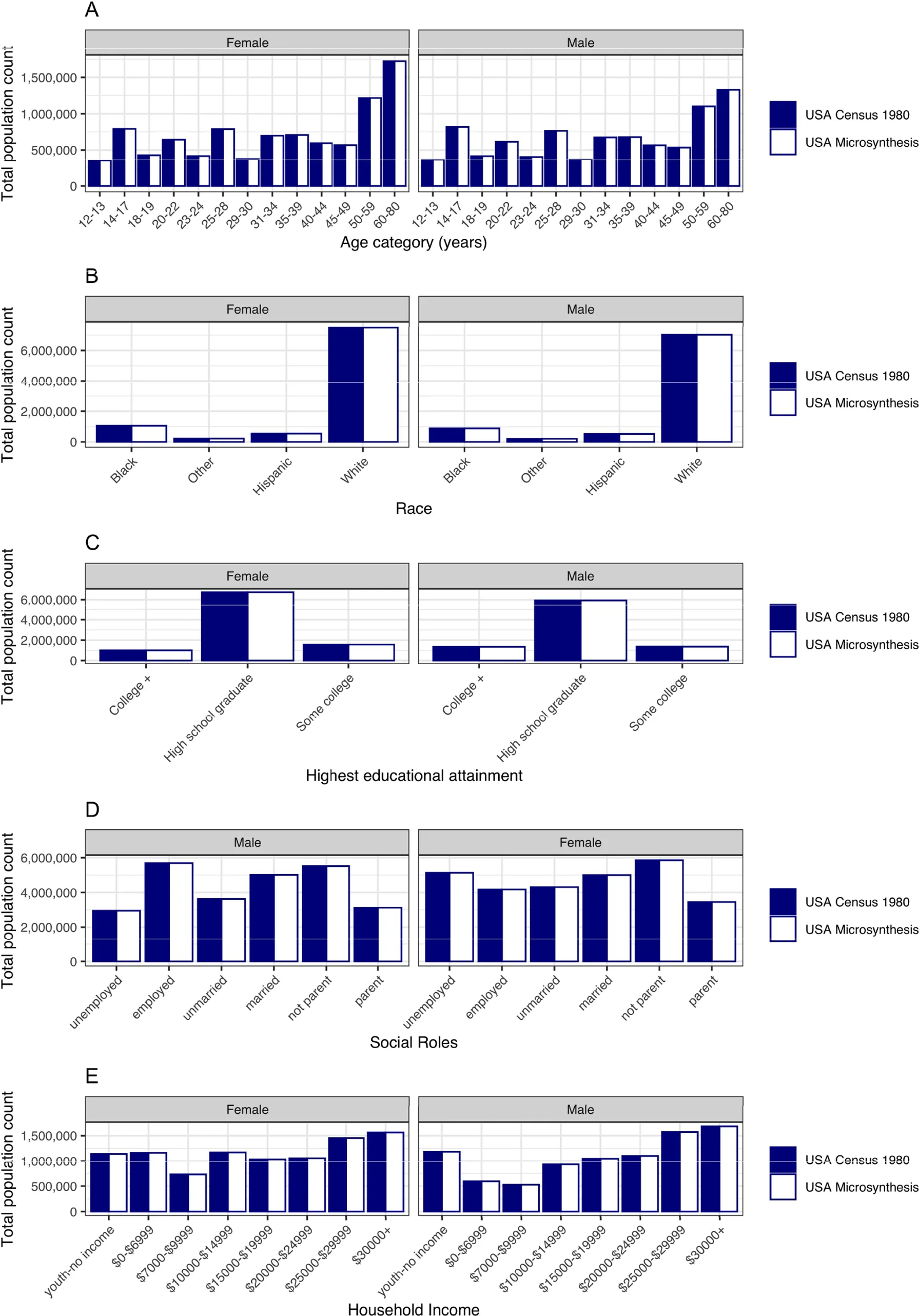
Table 2 and Figure 2 shows a comparison of the micro-synthetic population in the USA with the observed data from the 1980 Census. The comparisons show that the modeled numbers of males and females by age, race/ethnicity, education, employment status, marital status, parental status, and income category are all within 0.01% of the observed data. Similar results were found for CA, MN, NY, TN and TX, as a whole (shown in Appendix F).
| Female | Male | |||||
|---|---|---|---|---|---|---|
| Census | Micro-synthesis | Difference | Census | Micro-synthesis | Difference | |
| Age category | ||||||
| 12-13 | 350229 | 350205 | -0.007% | 363772 | 363800 | 0.009% |
| 14-17 | 791699 | 791646 | -0.007% | 819431 | 819457 | 0.003% |
| 18-19 | 428371 | 428374 | 0.001% | 416172 | 416174 | 0.001% |
| 20-22 | 643066 | 643061 | -0.001% | 614279 | 614288 | 0.001% |
| 23-24 | 417044 | 417041 | -0.001% | 404086 | 404082 | -0.001% |
| 25-28 | 788183 | 788182 | 0.001% | 764900 | 764913 | 0.002% |
| 29-30 | 377449 | 377447 | 0.001% | 366634 | 366636 | 0.001% |
| 31-34 | 698488 | 698489 | 0.001% | 673779 | 673785 | 0.001% |
| 35-39 | 708491 | 708494 | 0.001% | 678687 | 678684 | -0.001% |
| 40-44 | 594513 | 594520 | 0.001% | 565942 | 565942 | -0.001% |
| 45-49 | 568258 | 568258 | 0.001% | 534878 | 534884 | 0.001% |
| 50-59 | 1216357 | 1216358 | 0.001% | 1101383 | 1101380 | -0.001% |
| 60-80 | 1722769 | 1722765 | 0.001% | 1328453 | 1328450 | -0.001% |
| Race | ||||||
| Non-hispanic black | 1057394 | 1057385 | -0.001% | 884885 | 884883 | 0.001% |
| Hispanic | 538344 | 538341 | 0.001% | 519074 | 519080 | 0.001% |
| Non-hispanic other | 217081 | 217077 | -0.002% | 205423 | 205428 | 0.002% |
| Non-hispanic white | 7492101 | 7492037 | -0.001% | 7023014 | 7023084 | 0.001% |
| Education | ||||||
| High school graduate | 6737070 | 6736982 | -0.001% | 5927517 | 5927574 | 0.001% |
| Some college | 1565697 | 1565708 | 0.001% | 1361130 | 1361140 | 0.001% |
| College + | 1002151 | 1002150 | -0.001% | 1343748 | 1343761 | 0.001% |
| Social roles | ||||||
| Employed | 4172331 | 4172328 | 0.001% | 5688374 | 5688393 | 0.001% |
| Unemployed | 5132587 | 5132512 | -0.001% | 2944021 | 2944082 | 0.002% |
| Married | 4998998 | 4999000 | 0.000% | 5008429 | 5008440 | 0.000% |
| Unmarried | 4305920 | 4305840 | -0.002% | 3623966 | 3624035 | 0.002% |
| Not parent | 5854373 | 5854284 | -0.002% | 5510957 | 5511025 | 0.001% |
| Parent | 3450545 | 3450556 | 0.000% | 3121438 | 3121450 | 0.000% |
| Income category | ||||||
| $0-$6999 | 1162186 | 1162200 | 0.001% | 595240 | 595247 | 0.001% |
| $7000-$9999 | 728592 | 728572 | -0.003% | 525864 | 525871 | 0.001% |
| $10000-$14999 | 1170164 | 1170154 | -0.001% | 928740 | 928736 | 0.000% |
| $15000-$19999 | 1032560 | 1032568 | 0.001% | 1045736 | 1045737 | 0.000% |
| $20000-$24999 | 1054906 | 1054900 | -0.001% | 1100713 | 1100716 | 0.000% |
| $25000-$29999 | 1452311 | 1452312 | 0.000% | 1570514 | 1570508 | 0.000% |
| $30000+ | 1562268 | 1562283 | 0.001% | 1682380 | 1682403 | 0.001% |
| youth-no income | 1141928 | 1141851 | -0.007% | 1183202 | 1183257 | 0.005% |
Table 3 shows the detailed micro-synthesis breakdown by the 8 combinations of the three social roles (employment status, marital status, and parental status) for each state. For example, the micro-synthesis contains 4,300,758 individuals in CA aged 12-80 years who were employed AND married AND a parent. The available aggregate level Census does not report these specific combinations, but we can compare against the marginal totals for each role. Again, the percentage difference between modeled and observed is very small.
| California | Minnesota | New York | Tennessee | Texas | US | |
|---|---|---|---|---|---|---|
| Social Role Combination | ||||||
| _ _ _ | 399,495 | 65,449 | 333,353 | 77,874 | 220,355 | 3,864,726 |
| _ _ P | 60,378 | 5,848 | 53,551 | 10,807 | 29,980 | 522,189 |
| _ M _ | 209,202 | 42,456 | 189,861 | 54,541 | 122,314 | 2,439,605 |
| E _ _ | 335,976 | 53,877 | 228,962 | 49,159 | 170,089 | 2,782,588 |
| _ M P | 162,057 | 22,544 | 111,788 | 32,301 | 102,662 | 1,484,920 |
| E M _ | 201,329 | 42,494 | 142,986 | 43,569 | 141,361 | 2,119,030 |
| E _ P | 123,002 | 16,391 | 97,333 | 18,978 | 55,532 | 1,026,699 |
| E M P | 430,076 | 76,084 | 277,627 | 82,297 | 279,061 | 3,999,107 |
| % difference versus observed data | ||||||
| Married | 0.0001% | 0.0008% | 0.0003% | 0.0024% | 0.0009% | 0.0001% |
| Not married | 0.0001% | 0.0010% | 0.0003% | 0.0032% | 0.0012% | 0.0001% |
| Employed | 0.0001% | 0.0013% | 0.0002% | 0.0016% | 0.0003% | 0.0000% |
| Not Employed | 0.0001% | 0.0018% | 0.0002% | 0.0017% | 0.0004% | 0.0000% |
| Parent | 0.0003% | 0.0017% | 0.0004% | 0.0044% | 0.0008% | 0.0001% |
| Not Parent | 0.0002% | 0.0010% | 0.0003% | 0.0028% | 0.0005% | 0.0001% |
Notes: each possible combination using the abbreviations E – employed, M – married, P – parent, _ - not
3.2. Micro-synthesis model validation – the 1980 drinking patterns
Table 4 shows the estimated drinking patterns for the 1980 micro-synthesis in all six geographies. The prevalence of current drinkers (aged 12-80) ranged from 68.9% to 72.1%. The US national estimate was 70.3%, compared to the prevalence estimate based on NSDUH data of 73.0%. The frequency of alcohol use in the national micro-synthesis was 7.0 days in the past 30 days, compared to 6.8 based on NSDUH data. The mean quantity of alcohol consumed per day was estimated at 8.2 grams per day compared to 8.4 grams per day based on NSDUH. The model for heavy episodic drinking was the least close to the observed data with the mean number of 0.97 heavy drinking days in the past 30 days in the micro-synthesis compared to 0.88 days in the NSDUH US data – a difference of 9%. Table 4 also shows that the results vary by state and that the socio-demographics alter the estimated alcohol consumption patterns. There is no observed data from NSDUH representative at state level, therefore we were unable to undertake detailed state-level comparisons at this stage.
| State | Alcohol use prevalence | Mean alcohol use quantity (grams per day) | Mean alcohol use frequency (days per month) | Mean 5+ drink days per month |
|---|---|---|---|---|
| California | 72.17% | 8.22 | 7.04 | 0.95 |
| Minnesota | 72.14% | 8.38 | 7.07 | 0.98 |
| New York | 70.01% | 8.09 | 6.94 | 0.96 |
| Tennessee | 68.88% | 8.16 | 6.91 | 0.99 |
| Texas | 71.58% | 7.90 | 6.79 | 0.94 |
| USA | 70.33% | 8.18 | 6.97 | 0.97 |
| NSDUH, 2019 data | 72.96% [70.58, 75.33] | 8.44 [7.75, 9.13] | 6.88 [6.44, 7.31] | 0.88 [0.77, 0.99] |
3.3. Validation of the sociodemographic microsimulation over 30 years
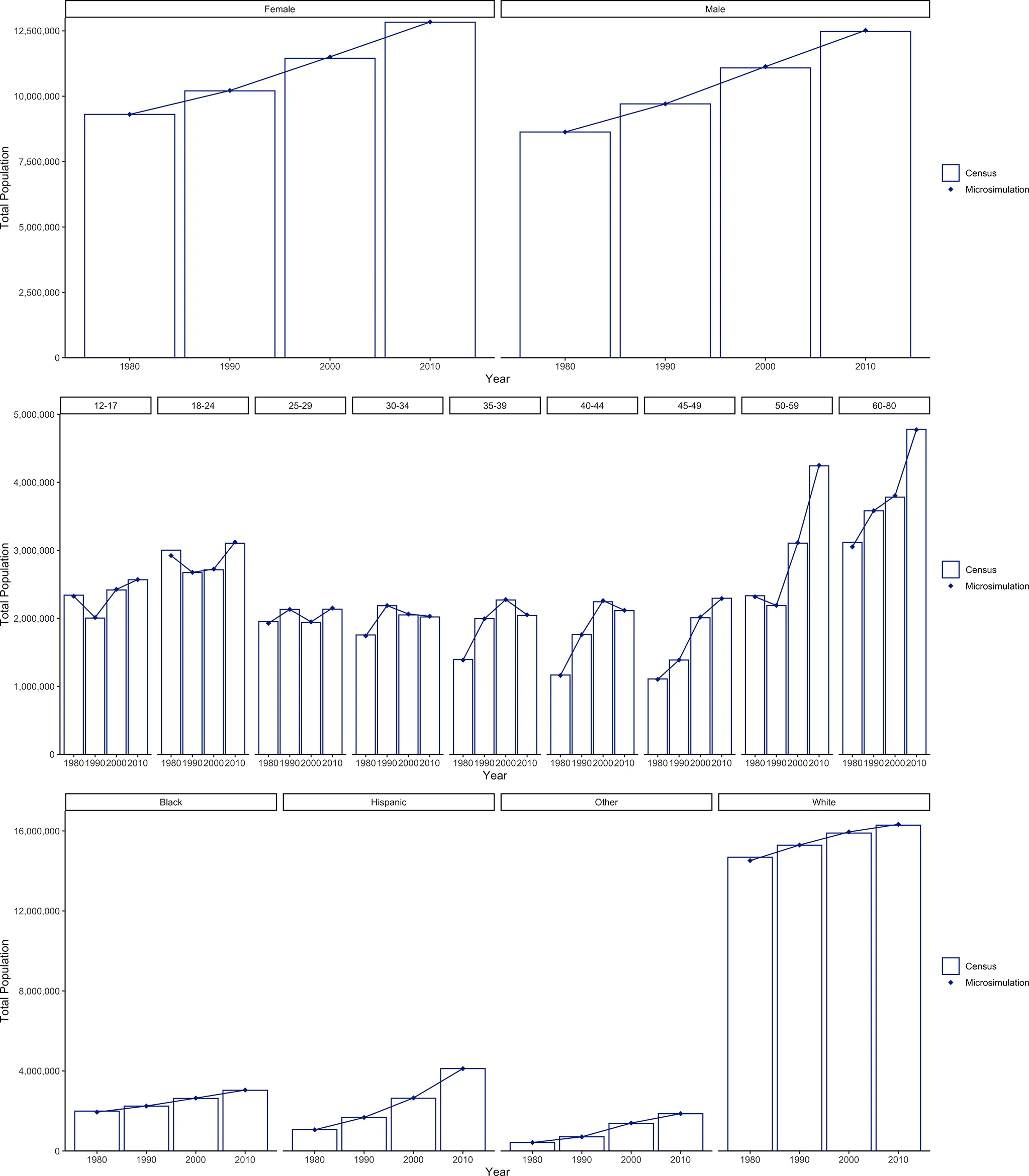
Figure 3 and Table 5 show the results of running the CASCADEPOP microsimulation for the USA over 30 years including the modeled dynamics for migration, births, and deaths. The population totals at the end of each decennial simulation year were compared against the corresponding Census data (1990, 2000, and 2010). The differences between the simulated population and the Census population were small for all comparisons undertaken for numbers of males and females, numbers in each of the nine age categories, and numbers of individuals in each of the four race/ethnicity groups - all of these being within 1.5% of the observed data across the whole 30-year simulation. The results for the other four states and for the US are similarly close (see Appendix G).
| 1990 | 2000 | 2010 | |||||||
|---|---|---|---|---|---|---|---|---|---|
| Census | Microsimulation | Difference | Census | Microsimulation | Difference | Census | Microsimulation | Difference | |
| Non-hispanic black | 2242309 | 2247300 | 0.22% | 2626753 | 2640870 | 0.54% | 3032982 | 3045380 | 0.41% |
| Hispanic | 1675274 | 1674900 | -0.02% | 2635389 | 2652050 | 0.63% | 4119840 | 4118710 | -0.03% |
| Non-hispanic other | 707779 | 708070 | 0.04% | 1377643 | 1394650 | 1.23% | 1861652 | 1865980 | 0.23% |
| Non-hispanic white | 15285788 | 15293890 | 0.05% | 15893199 | 15950070 | 0.36% | 16287723 | 16328920 | 0.25% |
| Female | 10204297 | 10217040 | 0.12% | 11450460 | 11505330 | 0.48% | 12828100 | 12838960 | 0.08% |
| Male | 9706853 | 9707120 | 0.00% | 11082530 | 11132310 | 0.45% | 12474100 | 12520030 | 0.37% |
| 12-17 | 2004212 | 2012300 | 0.40% | 2417936 | 2426610 | 0.36% | 2567835 | 2570450 | 0.10% |
| 18-24 | 2673777 | 2676540 | 0.10% | 2714345 | 2724760 | 0.38% | 3104722 | 3121590 | 0.54% |
| 25-29 | 2131305 | 2131710 | 0.02% | 1938134 | 1948060 | 0.51% | 2134600 | 2151870 | 0.81% |
| 30-34 | 2186289 | 2188090 | 0.08% | 2051039 | 2063780 | 0.62% | 2021027 | 2031350 | 0.51% |
| 35-39 | 1996312 | 1993430 | -0.14% | 2270666 | 2276720 | 0.27% | 2042091 | 2051510 | 0.46% |
| 40-44 | 1761579 | 1760510 | -0.06% | 2244186 | 2260780 | 0.74% | 2113322 | 2118880 | 0.26% |
| 45-49 | 1387257 | 1387940 | 0.05% | 2009240 | 2020340 | 0.55% | 2295657 | 2290950 | -0.21% |
| 50-59 | 2188227 | 2190440 | 0.10% | 3105479 | 3112160 | 0.22% | 4242635 | 4249330 | 0.16% |
| 60-80 | 3582194 | 3583200 | 0.03% | 3781961 | 3804430 | 0.59% | 4780309 | 4773060 | -0.15% |
3.4. Validation of the social roles microsimulation over 30 years
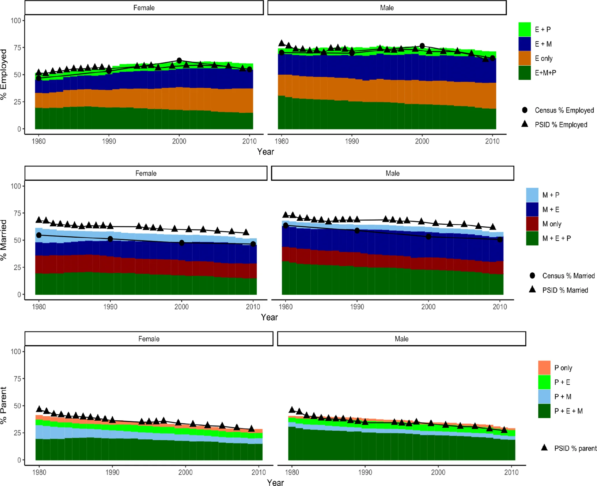
Figure 4 and Table 6 shows the results of running the CASCADEPOP social roles simulation for the USA between 1980 and 2010, applying the transition probabilities derived from PSID to each individual in each year of the simulation. The percentage of individuals employed and married were compared with Census data from 1980, 1990, 2000 and 2010, and parenting was compared with PSID data. Across all years of the simulation, the mean difference between modeled employment and Census data was 3.3% for women and 3.6% for men, the difference between modeled marriage and Census data was 5.8% for women and 6% for men. For parenting, the difference between the simulated and PSID data was 2.9% for women and 0.3% for men.
| Female | Male | |||||
|---|---|---|---|---|---|---|
| % | 1990 | 2000 | 2010 | 1990 | 2000 | 2010 |
| E only | 16.10 | 20.86 | 22.52 | 21.07 | 21.69 | 23.91 |
| E + M | 14.71 | 16.78 | 17.21 | 20.93 | 23.40 | 22.63 |
| E + P | 5.09 | 5.89 | 5.04 | 6.71 | 6.03 | 5.37 |
| E + M + P | 20.03 | 18.05 | 15.26 | 25.81 | 23.08 | 19.01 |
| Total Employed | 55.93 | 61.57 | 60.02 | 74.52 | 74.20 | 70.92 |
| Employed Census | 53.27 | 63.06 | 54.89 | 69.79 | 76.43 | 65.16 |
| Employed PSID | 55.51 | 57.57 | 55.22 | 71.64 | 73.14 | 63.89 |
| Difference (Microsimulation and Census) | 2.66 | -1.49 | 5.13 | 4.73 | -2.24 | 5.76 |
| M only | 15.37 | 13.83 | 13.64 | 13.45 | 11.47 | 12.11 |
| M + E | 14.71 | 16.78 | 17.21 | 20.93 | 23.40 | 22.63 |
| M + P | 7.60 | 5.86 | 5.11 | 3.66 | 3.81 | 3.43 |
| M + E + P | 20.03 | 18.05 | 15.26 | 25.81 | 23.08 | 19.01 |
| Total Married | 57.71 | 54.51 | 51.22 | 63.85 | 61.76 | 57.17 |
| Married Census | 51.18 | 47.58 | 46.45 | 58.89 | 53.23 | 50.59 |
| Married PSID | 62.51 | 59.97 | 56.67 | 68.55 | 66.75 | 61.61 |
| Difference (Microsimulation and census) | 6.53 | 6.93 | 4.77 | 4.97 | 8.52 | 6.58 |
| P only | 3.36 | 2.20 | 2.55 | 1.69 | 1.25 | 1.12 |
| P + E | 5.09 | 5.89 | 5.04 | 6.71 | 6.03 | 5.37 |
| P + M | 7.60 | 5.86 | 5.11 | 3.66 | 3.81 | 3.43 |
| P + E + M | 20.03 | 18.05 | 15.26 | 25.81 | 23.08 | 19.01 |
| Total Parent | 36.08 | 31.99 | 27.96 | 37.87 | 34.17 | 28.93 |
| Parent PSID | 36.24 | 33.87 | 28.16 | 34.29 | 33.27 | 27.07 |
| Difference (Microsimulation and PSID) | -0.16 | -1.88 | -0.20 | 3.58 | 0.90 | 1.86 |
4. Discussion
This study describes the methodology used to develop a US sociodemographic micro-synthesis and microsimulation over a 35-year period from 1980 to 2015 which can be used for a broad range of research questions in the fields of public health, epidemiology, demography, and policy analyses. This study demonstrated that CASCADEPOP v1.0 was able to generate a micro-synthesis (i.e., a synthetic baseline population) that accurately represents the sociodemographic structure of the 1980 populations of five different states and the US as a whole with regard to the joint distribution of age, sex, race/ethnicity, social roles (employment status, marital status, and parental status), education, and income. The 1980 drinking patterns simulated at baseline were also accurate. When the microsimulation was run forward in time, it reproduced demographic developments with regard to the age-sex-race/ethnicity structure of the US population over time.
Our work builds on the ideas of previous sociodemographic microsimulation approaches, in particular, the FRED (Grefenstette et al., 2013). However, with a much broader timeframe, rich sociodemographic characteristics and accurate sociodemographic developments over time CASCADEPOP can be used in numerous contexts with an expansive range of applications. We have developed methods to account for new entrants aged 12, deaths, and migration over an extended time period. To be able to accurately model sociodemographic changes over such a long period, as successfully tested in this operationalization of our approach, provides a platform for further modeling exercises. Our further work is now implementing agent-based models informed by several theories of what drives drinking decisions.
However, the CASCADEPOP platform and the microsimulation itself are not tied to simulations regarding alcohol use. Any population-representative survey with data on a behavior or risk factor, or combinations of behaviors and risk factors, could be utilized through the IPF process. This could include, for example, tobacco smoking, dietary behaviors, and physical activity measures. It could also include data on biomedical measures such as blood pressure, cholesterol, and blood sugars e.g. HbA1c as a measure of diabetes. Furthermore, if data sets are available to inform transition probabilities, dynamic changes in any of the implemented characteristics and behaviors can be modelled. In our application, we are using the microsimulation model to populate individuals into agent-based models and apply mechanisms to update drinking behavior. However, these mechanisms are not limited to this approach, and could be based on other methods including regression-based equations to update behavior of interest over time.
Here our model accounts for deaths from all-causes. In future work we intend to use our model to investigate mortality from specific causes that could be ameliorated by policy. To do this, we intend to calculate deaths from specific causes (i.e. liver cirrhosis, ICD-10 code 74) and subtract these from all-cause deaths to partition mortality into policy-modifiable and other causes. Other researchers can use our simulation to appraise a wide variety of policies from a number of diseases.
While modeling some of these additional risk factors may require additional sociodemographic variables to be included in the CASCADEPOP micro-synthesis and microsimulation. However, in developing our approach we were cognizant of many projects we have undertaken on epidemiological and health economic modeling in which the key variables have been age, sex, race/ethnicity, social roles, education, and income. The inclusion of all of these provides a strong basis for generalizable use of the platform. Furthermore, with all code being written in R and available as open-source, CASCADEPOP can be easily adjusted and modified. We will be seeking research funding to extend the tool across other nations, starting with the UK.
Limitations of our analysis are related to the datasets currently available and the requirements of IPF procedures. We are unable to examine the eight combinations of social roles against published census data because the census does not produce a report of a 3-way combination of employment status * marital status * parental status. We have compared, where possible, against marginal totals. A further challenge we have not been able to address is that religion is an important factor in explaining differences in drinking, but we have not found variables on religion in our key datasets that have been fit for the purpose, and so in version 1.0 of CASCADEPOP religion has been excluded. The IPF process does involve its own assumptions and produces a synthetic dataset by replicating records from the original dataset of interest used – in our case NSDUH. The NSDUH dataset utilized here is limited to data from 6105 respondents, containing some missing data points. As this paper is intended as a methodological description of the simulation, we have not imputed the missing data points, as the differences in alcohol consumption between missing and non-missing data were small, so would give a marginal benefit. As noted above, our microsimulation model is not tied to alcohol use, and others using other datasets may wish to explore imputation methods for missing data before the IPF procedure.
The social roles transition probabilities are only dependent on the age and sex of agents, and therefore cannot be used to generate more nuanced breakdowns of social role holding in society (i.e. differences by race/ethnicity or by education level). It was not possible for additional covariates to be added, as using 3 covariates for an 8-way transition matrix is already computationally intensive. Future work requiring a more nuanced description of role holding may utilize other approaches, such as regression modelling to develop transition rates dependent on several covariates.
We plan two substantial developments for CASCADEPOP version 2.0. The first and most important is that we plan to utilize a different exemplar dataset – the Behavioral Risk Factor Surveillance System (BRFSS). This contains data on health-related risk behaviors, chronic health conditions, and use of preventive services and was set up in 1984 with a large sample size, growing over time, with strong assessments of validity (Pierannunzi et al., 2013) and which has been used to study alcohol consumption behavior patterns (Delnevo et al., 2008). One limitation of self-reported alcohol consumption is that respondents often underestimate their consumption (Nelson et al., 2010). As part of this effort, we will also be relating reported levels of drinking in the survey to aggregate levels of sales data of alcohol, using methods to adjust individuals’ alcohol consumption so that the resulting synthetic population’s alcohol use is aligned with the reported sales (Meier et al., 2013; Rehm et al., 2010). Secondly, we will be further developing the dynamic sociodemographic variables to include income and education transitions.
The CASCADEPOP platform provides the capability to incorporate agent-based models that seek to explain and predict behaviors. We have already the first iteration of an agent-based model in which alcohol use is related to a theory of social norms (Probst et al., 2020). A similar model has also been developed which links alcohol use to the three social roles in a theory partly related to time available to drink given other responsibilities and partly to the stresses of having these roles (Bai et al., 2019; Vu et al., 2020a; Vu et al., 2020b). In each case, parameters theorized to be important in predicting drinking are estimated via a Bayesian calibration process (van der Vaart et al., 2015). This approach adjusted the parameters of the agent-based model so that the drinking behavior of individuals in the models matches historically observed alcohol consumption (i.e. from alcohol sales data). In future work, we also aim to calibrate our models to levels of alcohol related harms, namely liver cirrhosis and alcohol poisoning morbidity and mortality. A further key component of methodological development will be using genetic programming to alter features of the agent-based models and produce new model variants that could contain hybrid components of different theories to test whether they fit the observed data better than researcher defined theories and provide insights (Vu et al., 2019).
In summary, we have developed and validated a new sociodemographic microsimulation population model. The CASCADEPOP model can be used at State- and US-levels to simulate the evolution of populations and, when linked to data on behaviors and risk factors, can be used to analyze behaviors of public health significance.
Appendix
Alan Brennan, Charlotte Buckley, Tuong Manh Vu, Charlotte Probst, Alexandra Nielsen, Hao Bai, Thomas Broomhead, Thomas Greenfield, William Kerr, Petra S. Meier, Jurgen Rehm, Paul Shuper, Mark Strong, Robin C. Purshouse
A. Data preparation for Iterative Proportional Fitting using NSDUH, PSID and US Census 1980 to generate a base population for USA, California, New York, Texas, Tennessee, Minnesota.
104 cross-tabulated constraints were created based on age, race and sex, with 2 sex x 13 age x 4 race/ethnicity categories. Age is reported in individual years in the Census but to ensure that there were individuals belonging to each unique category in the individual level (PSID, NSDUH) datasets, ages were categorized. These categories were chosen to maximize granularity but ensure individual category membership and were comprised of the following: (12-13, 14-17, 18-19, 20-22, 23-24, 25-28, 29-30, 31-34, 35-39, 40-44, 45-49, 50-59, 60-80). Hispanic origin is categorized in NSDUH and PSID data as race, but ethnicity in the Census. As NSDUH and PSID don’t provide further breakdowns of race categories, all race categories from the Census not included in PSID or NSDUH datasets were classified as “other”. To get total population constraint counts, Census race categories were recoded into four categories reported in Table A1.
| Micro-synthetic population category | Census 1980 race categorizations |
|---|---|
| White (non-hispanic) | Not Spanish origin: white |
| Black (non-hispanic) | Not Spanish origin: black |
| Other (non-hispanic) | Not Spanish origin: American Indian, Eskimo, Aleut, Asian, Pacific Islander |
| Hispanic origin | Spanish Origin |
In the 1980 US Census, data is available on marriage status by sex for all individuals aged over 15 years. The following categories of marriage are available: single, married, separated, widowed, divorced. These were recoded into married (married) and unmarried (single, separated, widowed, divorced). Individuals under 15 years are assumed to be unmarried and the difference between the total population for each geography (based on the sex cross tabulation) and the total aged 15+ population was added to the unmarried category constraint for each group by sex. Employment status (“labor force status”) for men and women in the US census 1980 is available for all individuals over 16 years. As with marriage, individuals under the age of 16 are assumed to be unemployed and are added to the total count for unemployed individuals to make up the total population of each geography. The categories for employment are reported in Table A2.
| Micro-synthetic population category | Census 1980 employment categorizations |
|---|---|
| Employed | Labor force: employed |
| Unemployed | Labor force: unemployed, not in labor force |
Education in the Census is comprised of five categories. To ensure that all categories are consistent across datasets, we have re-categorized these into three broad categories of education level. These are: high school leaver and earlier, intermediate (corresponds to some college/some vocational or technical school) and college degree plus.
Household income data is expressed in categorical bands in earlier survey years (1979-2000) and in continuous $ in later years.
A.1. National Survey on Drug Use and Health (NSDUH) data processing
NSDUH data from 1979 was used to generate the base population for 1st January 1980. Variables used were sex, age, race, employment, parenthood and marital status, family income and education as well as the following alcohol variables: alcohol use prevalence (12 month), quantity (number of drinks per occasion), frequency (number of drinking occasions per month), heavy episodic drinking (number of 5+ drinks occasions per month).
A.2. Preparing NSDUH data for IPF
Variables were re-coded and re-categorized to be consistent with Census variables. Each variable to be used as a constraint for iterative proportional fitting was converted into binary form such that each participant represents a row, and each variable represents a column. Each row represents one survey respondent and each column a category which is being used as a constraint for the IPF. Respondents are assigned a 0 for categories they do not belong to and a 1 for categories which they do. Iterative proportional fitting was then used to create a matrix of individuals in geographic areas (States) and a weight was assigned to each individual from the microdata.
A.3. Panel Study of Income Dynamics (PSID) data processing
There are 14,982 individuals in the PSID dataset in 1979, a nationally representative sample of individuals in households in the USA. For the first stage Iterative Proportional Fitting, the following variables were used from the PSID data: age, sex, race/ethnicity (black, white, other, Hispanic origin). Marital status was inferred based on variables describing for each individual total number of marriages, and the years any marriages started and ended. This information was used to categorize individuals to be either married or unmarried. Employment status - there are several categorizations of employment in PSID employed, temporarily laid off, unemployed, retired, disabled, housewife, student, other. These were recoded into binary format to be employed and unemployed. Parenting is inferred based on whether individuals are the head of household, spouse or live in partner and whether there are children in the household under the age of 18.
B. Details on the steps for the micro-synthesis ipf for the base population
The goal of the micro-synthesis is to provide a simulated base population of individuals for the geography of interest. As an example, we want to have a micro-synthesis for the base California population on 1st January 1980 of N=18,957,712 aged 12 to 80. Therefore, we aim to have a database with over 18 million records which has the sociodemographic structure that matches the constraints.
A sequential set of steps is taken to incorporate the constraints from the five different datasets, making use of the Iterative Proportional Fitting ipfp package in R (Blocker, 2016), separately for each geography of interest (CA, MN, NY, TX, TN, USA). The process begins with our individual level dataset (NSDUH, 2019) which contains the drinking variables and socio-demographics described above. The sample size, after removing people who have missing required attributes, is n=6,105. The ipfp package is used to calculate a weight for each individual in the (NSDUH, 2019) dataset so that the re-weighted NSDUH has a sociodemographic structure that fits the known constraints of the geography of interest.
The micro-synthesis for CASCADEPOP v1.0 base population uses multiple constraints which are sourced from two datasets - the US census 1980 and the PSID 1980 datasets. In total, we use 138 constraints. There are 104 constraints for the three way cross-tabulation of 13 age categories / 2 sex / 4 race categories. There are 4 for marriage * sex. There are 4 for employment status * sex. There are 16 for 8 income categories * sex. There are 6 for education * sex.
The IPF procedure requires the following information:
A numeric constraint vector – one row per State (how many people in each demographic category), example Table B1.
Individual level dummy-coded constraint matrix – each row is a NSDUH individual, each column is a demographic category as in the constraint vector, example Table B2.
| Black 12-13 Female |
Black 12-13 Male |
Black 14-17 Female |
Black 14-17 Male |
|
|---|---|---|---|---|
| California | 33005 | 33216 | 74293 | 73992 |
| Black 12-13 Female |
Black 12-13 Male |
Black 14-17 Female |
Black 14-17 Male |
|
|---|---|---|---|---|
| NSDUH Individual 1 |
1 | 0 | 0 | 0 |
| NSDUH Individual 2 |
0 | 0 | 1 | 0 |
The IPF algorithm is then implemented using the ipfp package which reads in the numeric constraint vector in Table 1.4 and the individual constraint matrix Table 1.5. The weights are initially set to 1.
The IPF algorithm estimates a weight for each individual so that the total number of individuals in each of the 138 classified sociodemographic constraint categories matches the constraints Table 1.4. It iterates through different combinations of weights until it finds the best combination of weights.
The process goes through the 138 constraints 1.4 to reach the best solution. The modeller sets a tolerance level – we used a tolerance set to a very small number (10-10). Throughout the iterative process, this tolerance level is compared to a summary statistic of the error (L2 norm Euclidean distance between the vector of the reweighted population number and the constraint vector). The IPF model ‘converges’ when the L2 norm of error is below the tolerance level.
The iterative process proceeds as follows. The initial weight of 1 is multiplied by a ratio, with a the numerator that corresponds to the number of persons in this category in the constraints file, and a denominator that is the sum of the individuals in this category in the individual level data. For example, there are 33005 black, 12-13 year old females in the constraints data for California (Census 1980), whilst in the individual level 1979 NSDUH data, there are 43 individuals in this race, age, sex category. The weight for an individual in this category would be calculated as 33005/43=767.6. If the IPF was only based on the 3-way age/sex/race constraint, an individual in this category would receive a weight of 56.7. In reality, the process iterates through to try and find the best weight which represents the best fit for all of the constraint categories. In our example of 12-13 year old black females the real weights range between 767 and 768 for individuals in NSDUH weighted to the
California population. In our example, the IPF procedure produces estimated the weights in Table B3.
| NSDUH individual | California weight |
|---|---|
| Individual 1 | 5591.98 |
| Individual 2 | 2916.01 |
| Individual 3 | 3010.67 |
Table B3 indicates that individual 1 in the NSDUH dataset is representative of 5591.98 individuals in California. Note, this whole process is repeated for each State and in our example, the same NSDUH individual 1, had an estimated weight of and 5775.35 in Minnesota. This represents the best possible combination of weights for each individual such that the total constraints equal the known constraints of each geographical area. The final set of weights represents how many people each NSDUH individual represents for each of the US States. The weights generated are fractional and so cannot be used to create a table of individual level data. Therefore, these weights are converted to integers using the Truncate, Replicate, Sample (TRS) method (Lovelace and Ballas, 2013) which involves three steps:
Step 1) Truncate all non-integer weights by dropping the decimal place
Step 2) Replicate this number of individuals– using the example in Table B3 we would replicate 5591 individual 1’s, 2916 individual 2’s and 3010 individual 3’s into California.
Step 3) Sample to reach the correct number of people to account for (add back in) sum of all of the truncated decimal proportions of the weights. In our example for just 3 records in Table B3 this sums to 1.66. We round this to the nearest integer, which would be rounded to 2 in this case. Therefore 2 missing are then added to the dataset by randomly sampling from the NSUH individuals, using the leftover decimal for each individual to weight their probability of being sampled (so a person with truncated 0.99 is 99 times more likely to be sampled than a person with truncated 0.01). The result of this is that we now obtain the correct total population of Ca of N=18,957,712.
The final step is to append all of the required fields from individual 1 in NSDUH original dataset to each of the replicated versions of individual 1 in micro-synthetic dataset i.e. to ensure the micro-synthetic individuals have the correct alcohol use behaviour variables.
C. Data processing and method for creation of new migrants and 12 year olds for dynamic microsimulation
C.1. Migrants
Migration data downloaded from The Integrated Public Use Microdata Series (IPUMS USA). Data from the American Community Survey (ACS) 1990, 2000 and all years 2001-2015 (Ruggles et al., 2019). Individuals were determined as domestic (between-state) migrants based on their 5 year migration status (ACS 1990 and 2000) and 1 year migration status (ACS 2000+) and were determined as international migrants based on year of immigration variable (between 1980 and 2015). These years were used to determine the year the individual needs to enter the simulation. Individuals age at migration were determined by subtracting the difference between the survey year and migration year from the individuals age. Individuals were grouped in terms of migrants who had entered the state of interest and migrants who had left the state of interest by key demographic variables age, sex, race from the ACS. These individuals were then weighted based on the ACS person weight to get a representative number of migrants. When the data was based on 5-year migration status, the net migration was divided by 5 and allocated equally between surrounding years. The number of migrants who left in each age/sex/race category was subtracted from the number of migrants who entered each demographic category to produce a net migration value for each demographic category, in each state, in each year. The total count of migrants who entered the geography was then used as a constraint file for the IPF procedure.
C.2. 12-year olds
Using data from the US Census 1990, 2000, 2010, total counts of all individuals in each geographical area that were aged 21-12 in 1990, 2000, 2010 (to infer which individuals were 12 in 1981-1990, 1991-2000, 2001-2010), by race and sex. Some of these individuals will have been migrants that appeared in the census aged 12-21 in 1990, 2000, 2010. To avoid double counting these individuals as 12 year olds and migrants a crosscheck was calculated. This was done by calculating the age each migrant would have been when the decennial census occurred in 1990, 2000 and 2010. Any individual, which overlapped with a counted migrant, is then subtracted from the total count of twelve year olds. To estimate twelve year olds between 2011-2015, total counts of individuals aged 11,10,9,8 and 7 in the Census in 2010 by race/ethnicity were calculated, assuming that they would be turning 12 in 2011, 2012, 2013, 2014 and 2015, respectively.
C.3. IPF constraints
A constraints file for each year summarising the number of individuals which need to enter the model was created. This is based on the number of migrants which arrived in each geography that year and the number of individuals assumed to have been born and turned 12 during each year. This constraints file contained total counts for age, sex and race. New 12 year olds are assumed to be unemployed, unmarried, not parents and in the lowest education and income categories.
C.4. NSDUH data 1979-2016
The individual level data for migrants and 12 year olds entering the model each year was based on the closest NSDUH year to the year the individuals need to enter. NSDUH variables were harmonized in order to be comparable across survey years. These variables are: (1) Parenting status, whereby the variable names varied across survey years but broad categories remained the same (number of children under 18, or no children). In later NSDUH years this was expanded to include step-children. (2) Employment status, which became more detailed across survey years to include more categories, these were consistently recoded into employed versus unemployed with part-time employment being classified as employed.
C.5. Iterative proportional fitting
We used iterative proportional fitting to derive weights for NSDUH individuals from the closest survey year to the year they enter the model, based on the constraints file generated from the analysis of migrants and 12 year olds. The process was the same as described to generate the baseline population in Appendix B and results in a micro level dataset which contains information about individuals which need to enter the model for each year 1981 onwards including key demographics such as age, sex and race, social roles, income, education and alcohol behaviours from NSDUH.
D. Social roles transitions over time
| To | |||||||||
|---|---|---|---|---|---|---|---|---|---|
| Year period | From | _ _ _ | _ _ P | _ M _ | E _ _ | _ M P | E M _ | E _ P | E M P |
| 1979-1983 | _ _ _ | 5660 | 73 | 98 | 1670 | 2 | 117 | 32 | 2 |
| 1979-1983 | _ _ P | 50 | 984 | 1 | 19 | 70 | 0 | 357 | 7 |
| 1979-1983 | _ M _ | 187 | 0 | 9778 | 15 | 279 | 1040 | 0 | 114 |
| 1979-1983 | E _ _ | 1327 | 63 | 88 | 9229 | 4 | 683 | 188 | 33 |
| 1979-1983 | _ M P | 10 | 63 | 324 | 16 | 7123 | 125 | 35 | 2456 |
| 1979-1983 | E M _ | 25 | 13 | 1899 | 278 | 298 | 12523 | 25 | 987 |
| 1979-1983 | E _ P | 46 | 326 | 0 | 237 | 15 | 22 | 2256 | 110 |
| 1979-1983 | E M P | 8 | 14 | 123 | 91 | 1983 | 1127 | 237 | 22725 |
| 1984-1992 | _ _ _ | 7916 | 115 | 121 | 1924 | 20 | 142 | 87 | 4 |
| 1984-1992 | _ _ P | 91 | 1253 | 3 | 22 | 75 | 4 | 523 | 34 |
| 1984-1992 | _ M _ | 363 | 3 | 15513 | 86 | 332 | 1929 | 2 | 225 |
| 1984-1992 | E _ _ | 1954 | 66 | 108 | 14990 | 11 | 1027 | 418 | 58 |
| 1984-1992 | _ M P | 8 | 66 | 394 | 9 | 5680 | 134 | 37 | 3028 |
| 1984-1992 | E M _ | 67 | 2 | 2659 | 340 | 183 | 16588 | 14 | 1383 |
| 1984-1992 | E _ P | 35 | 562 | 4 | 300 | 36 | 19 | 3261 | 173 |
| 1984-1992 | E M P | 2 | 33 | 177 | 50 | 2663 | 1811 | 257 | 27641 |
| 1993-1999 | _ _ _ | 9464 | 86 | 98 | 1699 | 11 | 117 | 52 | 22 |
| 1993-1999 | _ _ P | 104 | 988 | 3 | 55 | 58 | 1 | 389 | 43 |
| 1993-1999 | _ M _ | 437 | 1 | 13984 | 41 | 181 | 1200 | 12 | 75 |
| 1993-1999 | E _ _ | 1561 | 74 | 95 | 13410 | 18 | 882 | 338 | 119 |
| 1993-1999 | _ M P | 7 | 44 | 291 | 15 | 3979 | 85 | 22 | 1661 |
| 1993-1999 | E M _ | 64 | 0 | 2096 | 438 | 180 | 18679 | 24 | 1109 |
| 1993-1999 | E _ P | 68 | 298 | 0 | 552 | 36 | 24 | 3600 | 187 |
| 1993-1999 | E M P | 8 | 37 | 97 | 104 | 1363 | 1560 | 300 | 21779 |
| 2000-2007 | _ _ _ | 8660 | 136 | 157 | 2108 | 54 | 197 | 131 | 139 |
| 2000-2007 | _ _ P | 257 | 624 | 14 | 114 | 68 | 2 | 332 | 54 |
| 2000-2007 | _ M _ | 1010 | 31 | 11729 | 96 | 219 | 1398 | 31 | 169 |
| 2000-2007 | E _ _ | 2119 | 122 | 159 | 12412 | 121 | 1258 | 580 | 660 |
| 2000-2007 | _ M P | 94 | 74 | 496 | 78 | 2709 | 329 | 97 | 1634 |
| 2000-2007 | E M _ | 227 | 15 | 3320 | 738 | 393 | 15780 | 59 | 1901 |
| 2000-2007 | E _ P | 138 | 311 | 23 | 823 | 52 | 160 | 2348 | 344 |
| 2000-2007 | E M P | 97 | 40 | 512 | 422 | 1339 | 3549 | 386 | 16740 |
| 2008-2015 | _ _ _ | 5660 | 73 | 98 | 1670 | 2 | 117 | 32 | 2 |
| 2008-2015 | _ _ P | 50 | 984 | 1 | 19 | 70 | 0 | 357 | 7 |
| 2008-2015 | _ M _ | 187 | 0 | 9778 | 15 | 279 | 1040 | 0 | 114 |
| 2008-2015 | E _ _ | 1327 | 63 | 88 | 9229 | 4 | 683 | 188 | 33 |
| 2008-2015 | _ M P | 10 | 63 | 324 | 16 | 7123 | 125 | 35 | 2456 |
| 2008-2015 | E M _ | 25 | 13 | 1899 | 278 | 298 | 12523 | 25 | 987 |
| 2008-2015 | E _ P | 46 | 326 | 0 | 237 | 15 | 22 | 2256 | 110 |
| 2008-2015 | E M P | 8 | 14 | 123 | 91 | 1983 | 1127 | 237 | 22725 |
| Transition | Baseline | Sex (male=1) | Age | Age squared | |
|---|---|---|---|---|---|
| 1979-1983 | _ _ _ > _ _ _ | -0.192 (-0.207, -0.178) | - | - | - |
| 1979-1983 | _ _ _ > _ _ P | 0.005 (0.004, 0.007) | 1.373 (1.231, 1.531) | 3.567 (1.912, 6.654) | 0.034 (0.015, 0.081) |
| 1979-1983 | _ _ _ > _ M _ | 0.015 (0.012, 0.019) | 0.944 (0.840, 1.062) | 0.703 (0.430, 1.149) | 0.585 (0.307, 1.113) |
| 1979-1983 | _ _ _ > E _ _ | 0.172 (0.158, 0.186) | 1.696 (1.584, 1.815) | 2.452 (1.942, 3.095) | 0.114 (0.085, 0.151) |
| 1979-1983 | _ _ P > _ _ _ | 0.053 (0.040, 0.072) | 0.963 (0.867, 1.070) | 17.507 (9.658, 31.733) | 0.193 (0.100, 0.373) |
| 1979-1983 | _ _ P > _ _ P | -0.227 (-0.252, -0.204) | - | - | - |
| 1979-1983 | _ _ P > _ M P | 0.029 (0.023, 0.038) | 0.944 (0.840, 1.062) | 0.703 (0.430, 1.149) | 0.585 (0.307, 1.113) |
| 1979-1983 | _ _ P > E _ P | 0.144 (0.129, 0.162) | 1.696 (1.584, 1.815) | 2.452 (1.942, 3.095) | 0.114 (0.085, 0.151) |
| 1979-1983 | _ M _ > _ _ _ | 0.022 (0.018, 0.026) | 0.531 (0.463, 0.608) | 0.068 (0.046, 0.101) | 14.837 (9.459, 23.271) |
| 1979-1983 | _ M _ > _ M _ | -0.231 (-0.244, -0.218) | - | - | - |
| 1979-1983 | _ M _ > _ M P | 0.040 (0.035, 0.047) | 0.802 (0.672, 0.957) | 0.018 (0.011, 0.030) | 14.050 (8.195, 24.089) |
| 1979-1983 | _ M _ > E M _ | 0.169 (0.158, 0.180) | 1.696 (1.584, 1.815) | 2.452 (1.942, 3.095) | 0.114 (0.085, 0.151) |
| 1979-1983 | E _ _ > _ _ _ | 0.220 (0.207, 0.234) | 0.544 (0.514, 0.575) | 0.024 (0.020, 0.028) | 93.597 (75.799, 115.573) |
| 1979-1983 | E _ _ > E _ _ | -0.259 (-0.274, -0.245) | - | - | - |
| 1979-1983 | E _ _ > E M _ | 0.036 (0.031, 0.042) | 0.944 (0.840, 1.062) | 0.703 (0.430, 1.149) | 0.585 (0.307, 1.113) |
| 1979-1983 | E _ _ > E _ P | 0.003 (0.003, 0.004) | 1.373 (1.231, 1.531) | 3.567 (1.912, 6.654) | 0.034 (0.015, 0.081) |
| 1979-1983 | _ M P > _ _ P | 0.009 (0.007, 0.012) | 0.531 (0.463, 0.608) | 0.068 (0.046, 0.101) | 14.837 (9.459, 23.271) |
| 1979-1983 | _ M P > _ M _ | 0.049 (0.043, 0.055) | 1.247 (1.044, 1.488) | 55.195 (33.654, 90.524) | 0.071 (0.042, 0.122) |
| 1979-1983 | _ M P > _ M P | -0.195 (-0.206, -0.185) | - | - | - |
| 1979-1983 | _ M P > E M P | 0.137 (0.129, 0.146) | 1.696 (1.584, 1.815) | 2.452 (1.942, 3.095) | 0.114 (0.085, 0.151) |
| 1979-1983 | E M _ > _ M _ | 0.280 (0.266, 0.294) | 0.544 (0.514, 0.575) | 0.024 (0.020, 0.028) | 93.597 (75.799, 115.573) |
| 1979-1983 | E M _ > E _ _ | 0.033 (0.029, 0.038) | 0.531 (0.463, 0.608) | 0.068 (0.046, 0.101) | 14.837 (9.459, 23.271) |
| 1979-1983 | E M _ > E M _ | -0.337 (-0.352, -0.321) | - | - | - |
| 1979-1983 | E M _ > E M P | 0.024 (0.020, 0.029) | 1.373 (1.231, 1.531) | 3.567 (1.912, 6.654) | 0.034 (0.015, 0.081) |
| 1979-1983 | E _ P > _ _ P | 0.308 (0.275, 0.345) | 0.544 (0.514, 0.575) | 0.024 (0.020, 0.028) | 93.597 (75.799, 115.573) |
| 1979-1983 | E _ P > E _ _ | 0.167 (0.144, 0.193) | 0.963 (0.867, 1.070) | 17.507 (9.658, 31.733) | 0.193 (0.100, 0.373) |
| 1979-1983 | E _ P > E _ P | -0.500 (-0.544, -0.460) | - | - | - |
| 1979-1983 | E _ P > E M P | 0.025 (0.020, 0.031) | 0.944 (0.840, 1.062) | 0.703 (0.430, 1.149) | 0.585 (0.307, 1.113) |
| 1979-1983 | E M P > _ M P | 0.254 (0.240, 0.270) | 0.544 (0.514, 0.575) | 0.024 (0.020, 0.028) | 93.597 (75.799, 115.573) |
| 1979-1983 | E M P > E M _ | 0.070 (0.062, 0.080) | 0.963 (0.867, 1.070) | 17.507 (9.658, 31.733) | 0.193 (0.100, 0.373) |
| 1979-1983 | E M P > E _ P | 0.020 (0.017, 0.023) | 0.531 (0.463, 0.608) | 0.068 (0.046, 0.101) | 14.837 (9.459, 23.271) |
| 1979-1983 | E M P > E M P | -0.345 (-0.363, -0.327) | - | - | - |
| 1984-1992 | _ _ _ > _ _ _ | -0.222 (-0.236 , -0.209) | - | - | - |
| 1984-1992 | _ _ _ > _ _ P | 0.010 (0.008, 0.012) | 1.315 (1.204, 1.436) | 10.677 (6.477, 17.601) | 0.010 (0.005, 0.020) |
| 1984-1992 | _ _ _ > _ M _ | 0.022 (0.019, 0.027) | 0.896 (0.813, 0.988) | 1.339 (0.900, 1.993) | 0.248 (0.146, 0.422) |
| 1984-1992 | _ _ _ > E _ _ | 0.190 (0.178, 0.204) | 1.972 (1.869, 2.080) | 3.950 (3.253, 4.797) | 0.071 (0.056, 0.089) |
| 1984-1992 | _ _ P > _ _ _ | 0.062 (0.050, 0.078) | 1.057 (0.970, 1.152) | 22.273 (12.836, 38.648) | 0.192 (0.104, 0.352) |
| 1984-1992 | _ _ P > _ _ P | -0.259 (-0.281, -0.238) | - | - | - |
| 1984-1992 | _ _ P > _ M P | 0.029 (0.023, 0.037) | 0.896 (0.813, 0.988) | 1.339 (0.900 1.993) | 0.248 (0.146, 0.422) |
| 1984-1992 | _ _ P > E _ P | 0.167 (0.152, 0.184) | 1.972 (1.869, 2.080) | 3.950 (3.253, 4.797) | 0.071 (0.056, 0.089) |
| 1984-1992 | _ M _ > _ _ _ | 0.031 (0.027, 0.035) | 0.557 (0.496, 0.626) | 0.086 (0.063, 0.117) | 10.938 (7.845, 15.252) |
| 1984-1992 | _ M _ > _ M _ | -0.272 (-0.285, -0.260) | - | - | - |
| 1984-1992 | _ M _ > _ M P | 0.037 (0.033, 0.043) | 1.132 (0.972, 1.317) | 0.010 (0.006, 0.015) | 23.864 (15.108, 37.697) |
| 1984-1992 | _ M _ > E M _ | 0.205 (0.194, 0.216) | 1.972 (1.869, 2.080) | 3.950 (3.253, 4.797) | 0.071 (0.056, 0.089) |
| 1984-1992 | E _ _ > _ _ _ | 0.217 (0.206, 0.229) | 0.695 (0.662, 0.729) | 0.057 (0.047, 0.068) | 36.814 (29.972, 45.219) |
| 1984-1992 | E _ _ > E _ _ | -0.253 (-0.265, -0.241) | - | - | - |
| 1984-1992 | E _ _ > E M _ | 0.031 (0.027, 0.036) | 0.896 (0.813, 0.988) | 1.339 (0.900, 1.993) | 0.248 (0.146, 0.422) |
| 1984-1992 | E _ _ > E _ P | 0.005 (0.004, 0.006) | 1.315 (1.204, 1.436) | 10.677 (6.477, 17.601) | 0.010 (0.005, 0.020) |
| 1984-1992 | _ M P > _ _ P | 0.012 (0.009, 0.015) | 0.557 (0.496, 0.626) | 0.086 (0.063, 0.117) | 10.938 (7.845, 15.252) |
| 1984-1992 | _ M P > _ M _ | 0.058 (0.051, 0.065) | 0.884 (0.759, 1.029) | 101.940 (66.119, 157.168) | 0.042 (0.027, 0.066) |
| 1984-1992 | _ M P > _ M P | -0.263 (-0.276, -0.251) | - | - | - |
| 1984-1992 | _ M P > E M P | 0.194 (0.184, 0.205) | 1.972 (1.869, 2.080) | 3.950 (3.253, 4.797) | 0.071 (0.056, 0.089) |
| 1984-1992 | E M _ > _ M _ | 0.271 (0.259, 0.284) | 0.695 (0.662, 0.729) | 0.057 (0.047, 0.068) | 36.814 (29.972, 45.219) |
| 1984-1992 | E M _ > E _ _ | 0.031 (0.028, 0.035) | 0.557 (0.496, 0.626) | 0.086 (0.063, 0.117) | 10.938 (7.845, 15.252) |
| 1984-1992 | E M _ > E M _ | -0.327 (-0.340, -0.314) | - | - | - |
| 1984-1992 | E M _ > E M P | 0.024 (0.021, 0.028) | 1.315 (1.204, 1.436) | 10.677 (6.477, 17.601) | 0.010 (0.005, 0.020) |
| 1984-1992 | E _ P > _ _ P | 0.349 (0.319, 0.382) | 0.695 (0.662, 0.729) | 0.057 (0.047, 0.068) | 36.814 (29.972, 45.219) |
| 1984-1992 | E _ P > E _ _ | 0.144 (0.125, 0.166) | 1.057 (0.970, 1.152) | 22.273 (12.836, 38.648) | 0.192 (0.104, 0.352) |
| 1984-1992 | E _ P > E _ P | -0.516 (-0.555, -0.481) | - | - | - |
| 1984-1992 | E _ P > E M P | 0.024 (0.020, 0.029) | 0.896 (0.813, 0.988) | 1.339 (0.900, 1.993) | 0.248 (0.146, 0.422) |
| 1984-1992 | E M P > _ M P | 0.253 (0.240, 0.267) | 0.695 (0.662, 0.729) | 0.057 (0.047, 0.068) | 36.814 (29.972, 45.219) |
| 1984-1992 | E M P > E M _ | 0.092 (0.082, 0.102) | 1.057 (0.970, 1.152) | 22.273 (12.836, 38.648) | 0.192 (0.104, 0.352) |
| 1984-1992 | E M P > E _ P | 0.014 (0.012, 0.016) | 0.557 (0.496, 0.626) | 0.086 (0.063, 0.117) | 10.938 (7.845, 15.252) |
| 1984-1992 | E M P > E M P | -0.359 (-0.376, -0.343) | - | - | - |
| 1993-1999 | _ _ _ > _ _ _ | -0.167 (-0.178, -0.156) | - | - | - |
| 1993-1999 | _ _ _ > _ _ P | 0.004 (0.003, 0.005) | 1.291 (1.175, 1.419) | 26.756 (14.879, 48.114) | 0.002 (0.001, 0.005) |
| 1993-1999 | _ _ _ > _ M _ | 0.012 (0.010, 0.015) | 1.068 (0.966, 1.181) | 0.809 (0.562, 1.165) | 0.525 (0.328, 0.841) |
| 1993-1999 | _ _ _ > E _ _ | 0.151 (0.140, 0.162) | 1.459 (1.369, 1.555) | 2.730 (2.251, 3.311) | 0.117 (0.094, 0.147) |
| 1993-1999 | _ _ P > _ _ _ | 0.070 (0.058, 0.085) | 1.195 (1.099, 1.299) | 26.429 (15.612, 44.741) | 0.097 (0.055, 0.173) |
| 1993-1999 | _ _ P > _ _ P | -0.273 (-0.297, -0.251) | - | - | - |
| 1993-1999 | _ _ P > _ M P | 0.037 (0.029, 0.047) | 1.068 (0.966, 1.181) | 0.809 (0.562, 1.165) | 0.525 (0.328, 0.841) |
| 1993-1999 | _ _ P > E _ P | 0.166 (0.149, 0.184) | 1.459 (1.369, 1.555) | 2.730 (2.251, 3.311) | 0.117 (0.094, 0.147) |
| 1993-1999 | _ M _ > _ _ _ | 0.029 (0.025, 0.033) | 0.610 (0.548, 0.678) | 0.074 (0.056, 0.099) | 12.452 (9.324, 16.628) |
| 1993-1999 | _ M _ > _ M _ | -0.226 (-0.238, -0.214) | - | - | - |
| 1993-1999 | _ M _ > _ M P | 0.037 (0.032, 0.042) | 0.889 (0.747, 1.059) | 0.020 (0.012, 0.033) | 13.229 (7.930, 22.067) |
| 1993-1999 | _ M _ > E M _ | 0.160 (0.150, 0.171) | 1.459 (1.369, 1.555) | 2.730 (2.251, 3.311) | 0.117 (0.094, 0.147) |
| 1993-1999 | E _ _ > _ _ _ | 0.145 (0.137, 0.154) | 0.652 (0.617, 0.690) | 0.040 (0.033, 0.048) | 45.233 (37.009, 55.285) |
| 1993-1999 | E _ _ > E _ _ | -0.182 (-0.191, -0.173) | - | - | - |
| 1993-1999 | E _ _ > E M _ | 0.033 (0.030, 0.037) | 1.068 (0.966, 1.181) | 0.809 (0.562, 1.165) | 0.525 (0.328, 0.841) |
| 1993-1999 | E _ _ > E _ P | 0.003 (0.003, 0.004) | 1.291 (1.175, 1.419) | 26.756 (14.879, 48.114) | 0.002 (0.001, 0.005) |
| 1993-1999 | _ M P > _ _ P | 0.011 (0.008, 0.014) | 0.610 (0.548, 0.678) | 0.074 (0.056, 0.099) | 12.452 (9.324, 16.628) |
| 1993-1999 | _ M P > _ M _ | 0.047 (0.041, 0.054) | 1.125 (0.945, 1.339) | 49.583 (30.151, 81.538) | 0.076 (0.045, 0.126) |
| 1993-1999 | _ M P > _ M P | -0.209 (-0.221, -0.198) | - | - | - |
| 1993-1999 | _ M P > E M P | 0.151 (0.142, 0.160) | 1.459 (1.369, 1.555) | 2.730 (2.251, 3.311) | 0.117 (0.094, 0.147) |
| 1993-1999 | E M _ > _ M _ | 0.151 (0.144, 0.159) | 0.652 (0.617, 0.690) | 0.040 (0.033, 0.048) | 45.233 (37.009, 55.285) |
| 1993-1999 | E M _ > E _ _ | 0.031 (0.028, 0.034) | 0.610 (0.548, 0.678) | 0.074 (0.056, 0.099) | 12.452 (9.324, 16.628) |
| 1993-1999 | E M _ > E M _ | -0.196 (-0.204, -0.187) | - | - | - |
| 1993-1999 | E M _ > E M P | 0.013 (0.011, 0.016) | 1.291 (1.175, 1.419) | 26.756 (14.879, 48.114) | 0.002 (0.001, 0.005) |
| 1993-1999 | E _ P > _ _ P | 0.158 (0.141, 0.177) | 0.652 (0.617, 0.690) | 0.040 (0.033, 0.048) | 45.233 (37.009, 55.285) |
| 1993-1999 | E _ P > E _ _ | 0.129 (0.115, 0.145) | 1.195 (1.099, 1.299) | 26.429 (15.612, 44.741) | 0.097 (0.055, 0.173) |
| 1993-1999 | E _ P > E _ P | -0.314 (-0.338, -0.292) | - | - | - |
| 1993-1999 | E _ P > E M P | 0.026 (0.022, 0.031) | 1.068 (0.966, 1.181) | 0.809 (0.562, 1.165) | 0.525 (0.328, 0.841) |
| 1993-1999 | E M P > _ M P | 0.131 (0.123, 0.140) | 0.652 (0.617, 0.690) | 0.040 (0.033, 0.048) | 45.233 (37.009, 55.285) |
| 1993-1999 | E M P > E M _ | 0.055 (0.049, 0.061) | 1.195 (1.099, 1.299) | 26.429 (15.612, 44.741) | 0.097 (0.055, 0.173) |
| 1993-1999 | E M P > E _ P | 0.020 (0.018, 0.023) | 0.610 (0.548, 0.678) | 0.074 (0.056, 0.099) | 12.452 (9.324, 16.628) |
| 1993-1999 | E M P > E M P | -0.207 (-0.218, -0.196) | - | - | - |
| 2000-2007 | _ _ _ > _ _ _ | -0.125 (-0.134, -0.118) | - | - | - |
| 2000-2007 | _ _ _ > _ _ P | 0.005 (0.004, 0.006) | 1.120 (1.029, 1.219) | 7.516 (4.755, 11.880) | 0.014 (0.008, 0.025) |
| 2000-2007 | _ _ _ > _ M _ | 0.011 (0.009, 0.013) | 1.010 (0.919, 1.111) | 2.309 (1.570, 3.396) | 0.132 (0.079, 0.221) |
| 2000-2007 | _ _ _ > E _ _ | 0.110 (0.102, 0.118) | 1.409 (1.320, 1.504) | 2.023 (1.682, 2.433) | 0.163 (0.132, 0.201) |
| 2000-2007 | _ _ P > _ _ _ | 0.104 (0.090, 0.120) | 1.019 (0.941, 1.103) | 91.910 (55.787, 151.423) | 0.036 (0.021, 0.059) |
| 2000-2007 | _ _ P > _ _ P | -0.238 (-0.259, -0.218) | - | - | - |
| 2000-2007 | _ _ P > _ M P | 0.023 (0.017, 0.030) | 1.010 (0.919, 1.111) | 2.309 (1.570, 3.396) | 0.132 (0.079, 0.221) |
| 2000-2007 | _ _ P > E _ P | 0.111 (0.098, 0.125) | 1.409 (1.320, 1.504) | 2.023 (1.682, 2.433) | 0.163 (0.132, 0.201) |
| 2000-2007 | _ M _ > _ _ _ | 0.021 (0.018, 0.024) | 0.593 (0.531, 0.661) | 0.151 (0.111, 0.207) | 6.699 (4.963, 9.043) |
| 2000-2007 | _ M _ > _ M _ | -0.203 (-0.214, -0.192) | - | - | - |
| 2000-2007 | _ M _ > _ M P | 0.036 (0.031, 0.042) | 0.901 (0.756, 1.073) | 0.026 (0.016, 0.043) | 8.191 (4.894, 13.710) |
| 2000-2007 | _ M _ > E M _ | 0.146 (0.137, 0.156) | 1.409 (1.320, 1.504) | 2.023 (1.682, 2.433) | 0.163 (0.132, 0.201) |
| 2000-2007 | E _ _ > _ _ _ | 0.095 (0.090, 0.101) | 0.759 (0.718, 0.802) | 0.064 (0.054, 0.077) | 21.372 (17.771, 25.702) |
| 2000-2007 | E _ _ > E _ _ | -0.125 (-0.131, -0.119) | - | - | - |
| 2000-2007 | E _ _ > E M _ | 0.024 (0.021, 0.026) | 1.010 (0.919, 1.111) | 2.309 (1.570, 3.396) | 0.132 (0.079, 0.221) |
| 2000-2007 | E _ _ > E _ P | 0.006 (0.005, 0.007) | 1.120 (1.029, 1.219) | 7.516 (4.755, 11.880) | 0.014 (0.008, 0.025) |
| 2000-2007 | _ M P > _ _ P | 0.016 (0.013, 0.021) | 0.593 (0.531, 0.661) | 0.151 (0.111, 0.207) | 6.699 (4.963, 9.043) |
| 2000-2007 | _ M P > _ M _ | 0.038 (0.033, 0.044) | 1.110 (0.932, 1.323) | 38.684 (23.429, 63.870) | 0.122 (0.073, 0.204) |
| 2000-2007 | _ M P > _ M P | -0.165 (-0.175, -0.156) | - | - | - |
| 2000-2007 | _ M P > E M P | 0.111 (0.104, 0.119) | 1.409 (1.320, 1.504) | 2.023 (1.682, 2.433) | 0.163 (0.132, 0.201) |
| 2000-2007 | E M _ > _ M _ | 0.109 (0.104, 0.115) | 0.759 (0.718, 0.802) | 0.064 (0.054, 0.077) | 21.372 (17.771, 25.702) |
| 2000-2007 | E M _ > E _ _ | 0.025 (0.023, 0.028) | 0.593 (0.531, 0.661) | 0.151 (0.111, 0.207) | 6.699 (4.963, 9.043) |
| 2000-2007 | E M _ > E M _ | -0.158 (-0.166, -0.152) | - | - | - |
| 2000-2007 | E M _ > E M P | 0.024 (0.021, 0.027) | 1.120 (1.029, 1.219) | 7.516 (4.755, 11.880) | 0.014 (0.008, 0.025) |
| 2000-2007 | E _ P > _ _ P | 0.112 (0.099, 0.126) | 0.759 (0.718, 0.802) | 0.064 (0.054, 0.077) | 21.372 (17.771, 25.702) |
| 2000-2007 | E _ P > E _ _ | 0.093 (0.084, 0.105) | 1.019 (0.941, 1.103) | 91.910 (55.787, 151.423) | 0.036 (0.021, 0.059) |
| 2000-2007 | E _ P > E _ P | -0.232 (-0.249, -0.215) | - | - | - |
| 2000-2007 | E _ P > E M P | 0.027 (0.023, 0.031) | 1.010 (0.919, 1.111) | 2.309 (1.570, 3.396) | 0.132 (0.079, 0.221) |
| 2000-2007 | E M P > _ M P | 0.079 (0.073, 0.084) | 0.759 (0.718, 0.802) | 0.064 (0.054, 0.077) | 21.372 (17.771, 25.702) |
| 2000-2007 | E M P > E M _ | 0.053 (0.048, 0.058) | 1.019 (0.941, 1.103) | 91.910 (55.787, 151.423) | 0.036 (0.021, 0.059) |
| 2000-2007 | E M P > E _ P | 0.013 (0.011, 0.015) | 0.593 (0.531, 0.661) | 0.151 (0.111, 0.207) | 6.699 (4.963, 9.043) |
| 2000-2007 | E M P > E M P | -0.144 (-0.152, -0.137) | - | - | - |
| 2008-2015 | _ _ _ > _ _ _ | -0.123 (-0.130, -0.116) | - | - | - |
| 2008-2015 | _ _ _ > _ _ P | 0.005 (0.004, 0.006) | 0.901 (0.814, 0.996) | 11.595 (6.733, 19.969) | 0.007 (0.004, 0.015) |
| 2008-2015 | _ _ _ > _ M _ | 0.007 (0.005, 0.008) | 0.959 (0.855, 1.076) | 3.233 (1.984, 5.266) | 0.092 (0.049, 0.174) |
| 2008-2015 | _ _ _ > E _ _ | 0.112 (0.105, 0.119) | 1.300 (1.225, 1.380) | 1.776 (1.488, 2.121) | 0.191 (0.156, 0.234) |
| 2008-2015 | _ _ P > _ _ _ | 0.114 (0.099, 0.132) | 1.130 (1.036, 1.231) | 23.441 (14.377, 38.219) | 0.122 (0.074, 0.203) |
| 2008-2015 | _ _ P > _ _ P | -0.261 (-0.284, -0.240) | - | - | - |
| 2008-2015 | _ _ P > _ M P | 0.018 (0.013, 0.024) | 0.959 (0.855, 1.076) | 3.233 (1.984, 5.266) | 0.092 (0.049, 0.174) |
| 2008-2015 | _ _ P > E _ P | 0.129 (0.115, 0.145) | 1.300 (1.225, 1.380) | 1.776 (1.488, 2.121) | 0.191 (0.156, 0.234) |
| 2008-2015 | _ M _ > _ _ _ | 0.036 (0.031, 0.040) | 0.572 (0.518, 0.632) | 0.053 (0.041, 0.068) | 14.804 (11.634, 18.839) |
| 2008-2015 | _ M _ > _ M _ | -0.198 (-0.209, -0.188) | - | - | - |
| 2008-2015 | _ M _ > _ M P | 0.029 (0.025, 0.034) | 0.856 (0.725, 1.011) | 0.051 (0.030, 0.087) | 5.022 (2.997, 8.414) |
| 2008-2015 | _ M _ > E M _ | 0.133 (0.125, 0.142) | 1.300 (1.225, 1.380) | 1.776 (1.488, 2.121) | 0.191 (0.156, 0.234) |
| 2008-2015 | E _ _ > _ _ _ | 0.117 (0.111, 0.123) | 0.780 (0.741, 0.822) | 0.110 (0.094, 0.128) | 12.971 (11.070, 15.199) |
| 2008-2015 | E _ _ > E _ _ | -0.135 (-0.141, -0.129) | - | - | - |
| 2008-2015 | E _ _ > E M _ | 0.015 (0.013, 0.017) | 0.959 (0.855, 1.076) | 3.233 (1.984, 5.266) | 0.092 (0.049, 0.174) |
| 2008-2015 | E _ _ > E _ P | 0.003 (0.003, 0.004) | 0.901 (0.814, 0.996) | 11.595 (6.733, 19.969) | 0.007 (0.004, 0.015) |
| 2008-2015 | _ M P > _ _ P | 0.010 (0.007, 0.014) | 0.572 (0.518, 0.632) | 0.053 (0.041, 0.068) | 14.804 (11.634, 18.839) |
| 2008-2015 | _ M P > _ M _ | 0.045 (0.039, 0.052) | 1.168 (0.989, 1.379) | 19.491 (11.548, 32.898) | 0.199 (0.119, 0.334) |
| 2008-2015 | _ M P > _ M P | -0.171 (-0.181, -0.161) | - | - | - |
| 2008-2015 | _ M P > E M P | 0.116 (0.108, 0.124) | 1.300 (1.225, 1.380) | 1.776 (1.488, 2.121) | 0.191 (0.156, 0.234) |
| 2008-2015 | E M _ > _ M _ | 0.111 (0.105, 0.117) | 0.780 (0.741, 0.822) | 0.110 (0.094, 0.128) | 12.971 (11.070, 15.199) |
| 2008-2015 | E M _ > E _ _ | 0.031 (0.028, 0.034) | 0.572 (0.518, 0.632) | 0.053 (0.041, 0.068) | 14.804 (11.634, 18.839) |
| 2008-2015 | E M _ > E M _ | -0.163 (-0.171, -0.156) | - | - | - |
| 2008-2015 | E M _ > E M P | 0.021 (0.018, 0.024) | 0.901 (0.814, 0.996) | 11.595 (6.733, 19.969) | 0.007 (0.004, 0.015) |
| 2008-2015 | E _ P > _ _ P | 0.130 (0.116, 0.146) | 0.780 (0.741, 0.822) | 0.110 (0.094, 0.128) | 12.971 (11.070, 15.199) |
| 2008-2015 | E _ P > E _ _ | 0.100 (0.089, 0.113) | 1.130 (1.036, 1.231) | 23.441 (14.377, 38.219) | 0.122 (0.074, 0.203) |
| 2008-2015 | E _ P > E _ P | -0.253 (-0.273, -0.234) | - | - | - |
| 2008-2015 | E _ P > E M P | 0.022 (0.019, 0.027) | 0.959 (0.855, 1.076) | 3.233 (1.984, 5.266) | 0.092 (0.049, 0.174) |
| 2008-2015 | E M P > _ M P | 0.079 (0.074, 0.085) | 0.780 (0.741, 0.822) | 0.110 (0.094, 0.128) | 12.971 (11.070, 15.199) |
| 2008-2015 | E M P > E M _ | 0.056 (0.051, 0.062) | 1.130 (1.036, 1.231) | 23.441 (14.377, 38.219) | 0.122 (0.074, 0.203) |
| 2008-2015 | E M P > E _ P | 0.019 (0.016, 0.021) | 0.572 (0.518, 0.632) | 0.053 (0.041, 0.068) | 14.804 (11.634, 18.839) |
| 2008-2015 | E M P > E M P | -0.154 (-0.163, -0.146) | - | - | - |
1_ =1 _ = not currently holding role, E= Employed, M = Married, P= Parent.
E. Microsimulation methodology and validation
We used empirical data to simulate the micro-synthesised population forwards in time using data from the ACS and Census to add new 12 year olds and migrants into the model and remove individuals due to migration and death. This was done by adding new micro-synthetic individuals, and applying rates to remove individuals from the model based on age, race/ethnicity and sex. This approach resulted in the micro-simulated population representing 97.6% of the total census population by 1990 (reported for California). However, some individual demographic categories were over, and underestimated. Table E1 shows a summary of differences between the micro-simulated and Census population of California for 1990.
| California 1990 | Total | Male | Female | Black | White | Hispanic | Other |
|---|---|---|---|---|---|---|---|
| Micro-simulated population | 2346930 | 1174600 | 1172330 | 196620 | 1449040 | 475800 | 225470 |
| Census population | 2372956 | 1191852 | 1181104 | 163098 | 1403873 | 570837 | 235147 |
| % difference | -1.1% | -1.4% | -0.7% | +20.5% | +3.2% | -16.6% | -4.1% |
Notes: positive values indicate that the microsimulation has over-estimated. Negative values indicate the microsimulation has under estimated.
There are several candidate explanations for this modelled difference. First, the ACS weights may not fully represent all migrants between states, and may also fail to fully capture data on migration from specific states to abroad. The definition of Black and Hispanic in the census is also inconsistent across ACS and Census years, and further detailed categories were introduced in later years and therefore individuals may have had more options to self-categorize and may have changed between our race/ethnicity bands. As shown in Table E1, the error is different for each category. Therefore, a smoothing procedure was undertaken to account for this error and unknown migration rates so that the populations in 1990, 2000 and 2010 correspond to the most accurate (Census) representation of the age/sex/race demographic of each state.
This procedure calculated the difference between the modelled population and the population in each Census year, and adjusted the outward migration rates across the previous 10 years to remove the correct number of individuals and result in the correct population in each State in each Census year. For example, if our micro-simulated population contained 100 individuals more than the census population, we would remove 10 individuals from each category in each of the previous 10 years of the simulation. For demographic categories under-estimated in the microsimulation, the migration IPF constraints were adjusted for each year to ensure the correct demographic profile in each Census year. This adjustment consisted of missing individuals being added to the IPF constraints equally to arrive at the correct population total count in each Census year. In a similar process to the adjustment of outward migration rates, if there were 100 individuals too few in the microsimulation compared to Census, then we added 10 individuals onto the migration constraints for each year leading up to that census year. The adjustment of the migration in and out rates also accounted for ageing, if there were 100 too many 30 year old’s in 1990, we would remove 10 29-year-olds from 1989, 10 28-year-olds from 1988, and so forth.
F. Validation of demographics for the baseline microsynthesis population in California, Minnesota, New York, Tennessee and Texas in 1980.
| Female | Male | |||||
|---|---|---|---|---|---|---|
| Census | Micro-synthesis | % difference | Census | Micro-synthesis | % difference | |
| 12-13 | 34319 | 34321 | -0.01% | 35516 | 35516 | -0.01% |
| 14-17 | 78235 | 78235 | -0.01% | 80271 | 80265 | 0.00% |
| 18-19 | 43149 | 43149 | 0.00% | 42496 | 42495 | 0.01% |
| 20-22 | 67427 | 67427 | 0.00% | 67082 | 67081 | 0.00% |
| 23-24 | 46233 | 46234 | 0.00% | 46481 | 46482 | 0.00% |
| 25-28 | 88104 | 8813 | 0.00% | 88702 | 88702 | 0.00% |
| 29-30 | 42761 | 42761 | 0.00% | 42895 | 42896 | 0.00% |
| 31-34 | 78497 | 78497 | 0.00% | 77893 | 77893 | 0.00% |
| 35-39 | 77326 | 77327 | 0.00% | 76723 | 76724 | 0.00% |
| 40-44 | 63134 | 63133 | 0.00% | 62340 | 62340 | 0.00% |
| 45-49 | 58371 | 58372 | 0.00% | 57422 | 57422 | 0.00% |
| 50-59 | 124046 | 124046 | 0.00% | 114417 | 114418 | 0.00% |
| 60-80 | 162490 | 162492 | 0.00% | 129435 | 129435 | 0.00% |
| Black | 71332 | 71333 | 0.00% | 63901 | 63901 | 0.00% |
| Hispanic | 162686 | 162687 | 0.00% | 163695 | 163696 | 0.00% |
| Other | 63678 | 63678 | -0.01% | 60735 | 60736 | 0.00% |
| White | 666395 | 666398 | 0.00% | 633346 | 633341 | 0.00% |
| High school graduate | 641079 | 641084 | 0.00% | 549945 | 549939 | 0.00% |
| Some college | 202229 | 202231 | 0.00% | 198391 | 198391 | 0.00% |
| College + | 120782 | 120780 | 0.00% | 173343 | 173344 | 0.00% |
| employed | 456422 | 456420 | 0.000% | 622114 | 622114 | 0.000% |
| unemployed | 507669 | 507675 | 0.001% | 299565 | 299560 | -0.002% |
| married | 496685 | 496686 | 0.000% | 501221 | 501222 | 0.000% |
| unmarried | 467406 | 467410 | 0.001% | 420458 | 420452 | -0.001% |
| not parent | 587778 | 587782 | 0.001% | 572818 | 572811 | -0.001% |
| parent | 376313 | 376314 | 0.000% | 348861 | 348863 | 0.000% |
| $0-$6999 | 116207 | 116208 | 0.001% | 63197 | 63196 | -0.001% |
| $7000-$9999 | 73902 | 73904 | 0.002% | 56098 | 56099 | 0.002% |
| $10000-$14999 | 132318 | 132317 | 0.000% | 97953 | 97953 | 0.000% |
| $15000-$19999 | 105334 | 105334 | 0.000% | 110883 | 110882 | -0.002% |
| $20000-$24999 | 111145 | 111145 | 0.000% | 118663 | 118664 | 0.001% |
| $25000-$29999 | 151786 | 151784 | -0.001% | 171233 | 171234 | 0.000% |
| $30000+ | 160845 | 160845 | 0.000% | 187861 | 187862 | 0.001% |
| youth-no income | 112554 | 112556 | 0.003% | 115788 | 115781 | -0.006% |
| Female | Male | |||||
|---|---|---|---|---|---|---|
| Census | Micro-synthesis | % difference | Census | Micro-synthesis | % difference | |
| 12-13 | 27241 | 27238 | -0.01% | 28255 | 28253 | -0.01% |
| 14-17 | 61564 | 61556 | -0.01% | 63441 | 63440 | 0.00% |
| 18-19 | 32127 | 32128 | 0.00% | 30794 | 30796 | 0.01% |
| 20-22 | 47405 | 47406 | 0.00% | 43889 | 43890 | 0.00% |
| 23-24 | 30533 | 30533 | 0.00% | 28029 | 28030 | 0.00% |
| 25-28 | 58583 | 58584 | 0.00% | 54319 | 54320 | 0.00% |
| 29-30 | 29450 | 29451 | 0.00% | 27114 | 27114 | 0.00% |
| 31-34 | 55495 | 55496 | 0.00% | 50642 | 50643 | 0.00% |
| 35-39 | 57839 | 57841 | 0.00% | 52096 | 52096 | 0.00% |
| 40-44 | 48834 | 48835 | 0.00% | 44256 | 44256 | 0.00% |
| 45-49 | 47692 | 47692 | 0.00% | 42947 | 42948 | 0.00% |
| 50-59 | 104535 | 104537 | 0.00% | 91546 | 91545 | 0.00% |
| 60-80 | 147327 | 147327 | 0.00% | 107702 | 107703 | 0.00% |
| Black | 99616 | 99617 | 0.00% | 77367 | 77368 | 0.00% |
| Hispanic | 67549 | 67549 | 0.00% | 56821 | 56820 | 0.00% |
| Other | 16987 | 16986 | -0.01% | 16640 | 16640 | 0.00% |
| White | 564477 | 564474 | 0.00% | 514208 | 514209 | 0.00% |
| High school graduate | 529602 | 529597 | 0.00% | 443144 | 443145 | 0.00% |
| Some college | 125710 | 125712 | 0.00% | 104317 | 104318 | 0.00% |
| College + | 93318 | 93319 | 0.00% | 117574 | 117576 | 0.00% |
| employed | 82042 | 82039 | -0.004% | 106867 | 106868 | 0.001% |
| unemployed | 81373 | 81373 | -0.001% | 49791 | 49794 | 0.006% |
| married | 91259 | 91256 | -0.003% | 91588 | 91588 | 0.000% |
| unmarried | 72157 | 72155 | -0.002% | 65070 | 65074 | 0.006% |
| not parent | 104887 | 104886 | -0.001% | 100877 | 100881 | 0.003% |
| parent | 58529 | 58526 | -0.005% | 55781 | 55781 | 0.001% |
| $0-$6999 | 16634 | 16632 | -0.008% | 9321 | 9321 | -0.009% |
| $7000-$9999 | 11580 | 11579 | -0.014% | 8827 | 8827 | 0.000% |
| $10000-$14999 | 19356 | 19357 | 0.004% | 16283 | 16283 | -0.004% |
| $15000-$19999 | 18250 | 18249 | -0.008% | 18769 | 18769 | -0.003% |
| $20000-$24999 | 18958 | 18958 | -0.002% | 20074 | 20075 | 0.005% |
| $25000-$29999 | 27461 | 27461 | 0.000% | 29382 | 29382 | 0.001% |
| $30000+ | 29991 | 29990 | -0.003% | 31826 | 31827 | 0.002% |
| youth-no income | 21183 | 21184 | 0.005% | 22172 | 22176 | 0.018% |
| Female | Male | |||||
|---|---|---|---|---|---|---|
| Census | Micro-synthesis | % difference | Census | Micro-synthesis | % difference | |
| 12-13 | 27241 | 27238 | -0.01% | 28255 | 28253 | -0.01% |
| 14-17 | 61564 | 61556 | -0.01% | 63441 | 63440 | 0.00% |
| 18-19 | 32127 | 32128 | 0.00% | 30794 | 30796 | 0.01% |
| 20-22 | 47405 | 47406 | 0.00% | 43889 | 43890 | 0.00% |
| 23-24 | 30533 | 30533 | 0.00% | 28029 | 28030 | 0.00% |
| 25-28 | 58583 | 58584 | 0.00% | 54319 | 54320 | 0.00% |
| 29-30 | 29450 | 29451 | 0.00% | 27114 | 27114 | 0.00% |
| 31-34 | 55495 | 55496 | 0.00% | 50642 | 50643 | 0.00% |
| 35-39 | 57839 | 57841 | 0.00% | 52096 | 52096 | 0.00% |
| 40-44 | 48834 | 48835 | 0.00% | 44256 | 44256 | 0.00% |
| 45-49 | 47692 | 47692 | 0.00% | 42947 | 42948 | 0.00% |
| 50-59 | 104535 | 104537 | 0.00% | 91546 | 91545 | 0.00% |
| 60-80 | 147327 | 147327 | 0.00% | 107702 | 107703 | 0.00% |
| Black | 99616 | 99617 | 0.00% | 77367 | 77368 | 0.00% |
| Hispanic | 67549 | 67549 | 0.00% | 56821 | 56820 | 0.00% |
| Other | 16987 | 16986 | -0.01% | 16640 | 16640 | 0.00% |
| White | 564477 | 564474 | 0.00% | 514208 | 514209 | 0.00% |
| High school graduate | 529602 | 529597 | 0.00% | 443144 | 443145 | 0.00% |
| Some college | 125710 | 125712 | 0.00% | 104317 | 104318 | 0.00% |
| College + | 93318 | 93319 | 0.00% | 117574 | 117576 | 0.00% |
| employed | 324473 | 324476 | 0.001% | 421505 | 421509 | 0.001% |
| unemployed | 424158 | 424151 | -0.002% | 243530 | 243530 | 0.000% |
| married | 360180 | 360187 | 0.002% | 360048 | 360051 | 0.001% |
| unmarried | 388451 | 388441 | -0.003% | 304988 | 304988 | 0.000% |
| not parent | 478148 | 478139 | -0.002% | 433012 | 433013 | 0.000% |
| parent | 270483 | 270488 | 0.002% | 232024 | 232026 | 0.001% |
| $0-$6999 | 105097 | 105099 | 0.001% | 50391 | 50391 | 0.001% |
| $7000-$9999 | 63228 | 63228 | -0.001% | 41904 | 41904 | 0.001% |
| $10000-$14999 | 98860 | 98863 | 0.003% | 72189 | 72191 | 0.002% |
| $15000-$19999 | 81467 | 81469 | 0.001% | 79584 | 79585 | 0.001% |
| $20000-$24999 | 81939 | 81940 | 0.001% | 82614 | 82615 | 0.002% |
| $25000-$29999 | 110219 | 110219 | 0.000% | 118694 | 118694 | 0.000% |
| $30000+ | 119011 | 119013 | 0.002% | 127961 | 127963 | 0.001% |
| youth-no income | 88805 | 88794 | -0.013% | 91696 | 91694 | -0.003% |
| Female | Male | |||||
|---|---|---|---|---|---|---|
| Census | Micro-synthesis | % difference | Census | Micro-synthesis | % difference | |
| 12-13 | 7062 | 7062 | -0.01% | 7376 | 7375 | -0.01% |
| 14-17 | 16008 | 16011 | -0.01% | 16635 | 16633 | 0.00% |
| 18-19 | 8663 | 8663 | 0.00% | 8392 | 8392 | 0.01% |
| 20-22 | 12939 | 12939 | 0.00% | 12203 | 12203 | 0.00% |
| 23-24 | 8385 | 8386 | 0.00% | 7934 | 7935 | 0.00% |
| 25-28 | 15954 | 15953 | 0.00% | 15000 | 14999 | 0.00% |
| 29-30 | 7568 | 7567 | 0.00% | 7283 | 7283 | 0.00% |
| 31-34 | 14319 | 14319 | 0.00% | 13590 | 13591 | 0.00% |
| 35-39 | 14687 | 14687 | 0.00% | 13948 | 13948 | 0.00% |
| 40-44 | 12653 | 12653 | 0.00% | 11861 | 11861 | 0.00% |
| 45-49 | 12032 | 12033 | 0.00% | 10884 | 10883 | 0.00% |
| 50-59 | 24527 | 24527 | 0.00% | 21601 | 21601 | 0.00% |
| 60-80 | 35567 | 35566 | 0.00% | 26752 | 26752 | 0.00% |
| Black | 29365 | 29365 | 0.00% | 23977 | 23978 | 0.00% |
| Hispanic | 1347 | 1347 | 0.00% | 1227 | 1226 | 0.00% |
| Other | 969 | 969 | -0.01% | 919 | 920 | 0.00% |
| White | 158686 | 158691 | 0.00% | 147339 | 147335 | 0.00% |
| High school graduate | 148035 | 148038 | 0.00% | 131070 | 131067 | 0.00% |
| Some college | 25913 | 25913 | 0.00% | 21497 | 21496 | 0.00% |
| College + | 16420 | 16420 | 0.00% | 20896 | 20897 | 0.00% |
| employed | 82113 | 82113 | 0.000% | 110522 | 110523 | 0.000% |
| unemployed | 108255 | 108259 | 0.004% | 62942 | 62937 | -0.007% |
| married | 105877 | 105877 | 0.000% | 105925 | 105924 | 0.000% |
| unmarried | 84491 | 84495 | 0.005% | 67539 | 67535 | -0.006% |
| not parent | 118870 | 118873 | 0.003% | 110051 | 110048 | -0.003% |
| parent | 71498 | 71499 | 0.001% | 63413 | 63412 | -0.001% |
| $0-$6999 | 24557 | 24556 | -0.004% | 12456 | 12456 | -0.004% |
| $7000-$9999 | 15018 | 15019 | 0.003% | 10596 | 10596 | 0.001% |
| $10000-$14999 | 22960 | 22961 | 0.005% | 18886 | 18886 | 0.001% |
| $15000-$19999 | 21447 | 21447 | 0.000% | 21310 | 21310 | 0.001% |
| $20000-$24999 | 21576 | 21575 | -0.003% | 22217 | 22217 | -0.001% |
| $25000-$29999 | 29785 | 29786 | 0.003% | 31355 | 31354 | -0.004% |
| $30000+ | 31952 | 31951 | -0.002% | 32629 | 32629 | 0.002% |
| youth-no income | 23070 | 23074 | 0.018% | 24012 | 24008 | -0.013% |
| Female | Male | |||||
|---|---|---|---|---|---|---|
| Census | Micro-synthesis | % difference | Census | Micro-synthesis | % difference | |
| 12-13 | 22357 | 22358 | -0.01% | 23270 | 23271 | -0.01% |
| 14-17 | 49894 | 49898 | -0.01% | 51592 | 51585 | 0.00% |
| 18-19 | 27180 | 27179 | 0.00% | 26834 | 26834 | 0.01% |
| 20-22 | 41451 | 41451 | 0.00% | 40474 | 40475 | 0.00% |
| 23-24 | 27802 | 27802 | 0.00% | 27631 | 27631 | 0.00% |
| 25-28 | 52002 | 52003 | 0.00% | 51844 | 51844 | 0.00% |
| 29-30 | 24265 | 24264 | 0.00% | 24162 | 24163 | 0.00% |
| 31-34 | 44007 | 44006 | 0.00% | 43471 | 43469 | 0.00% |
| 35-39 | 44166 | 44166 | 0.00% | 43097 | 43098 | 0.00% |
| 40-44 | 36665 | 36664 | 0.00% | 35275 | 35276 | 0.00% |
| 45-49 | 34670 | 34670 | 0.00% | 33095 | 33095 | 0.00% |
| 50-59 | 68693 | 68694 | 0.00% | 62974 | 62974 | 0.00% |
| 60-80 | 91746 | 91746 | 0.00% | 72024 | 72025 | 0.00% |
| Black | 66501 | 66499 | 0.00% | 57637 | 57639 | 0.00% |
| Hispanic | 107300 | 107300 | 0.00% | 103714 | 103715 | 0.00% |
| Other | 7612 | 7612 | -0.01% | 7592 | 7591 | 0.00% |
| White | 383487 | 383493 | 0.00% | 366805 | 366799 | 0.00% |
| employed | 261540 | 261539 | 0.000% | 378302 | 378304 | 0.001% |
| unemployed | 303362 | 303367 | 0.002% | 157447 | 157441 | -0.004% |
| married | 320345 | 320344 | 0.000% | 322254 | 322255 | 0.000% |
| unmarried | 244557 | 244562 | 0.002% | 213495 | 213490 | -0.002% |
| not parent | 337557 | 337565 | 0.002% | 326571 | 326565 | -0.002% |
| parent | 227344 | 227341 | -0.001% | 209179 | 209180 | 0.001% |
| $0-$6999 | 66610 | 66610 | 0.001% | 33977 | 33979 | 0.005% |
| $7000-$9999 | 43731 | 43730 | -0.003% | 33648 | 33649 | 0.003% |
| $10000-$14999 | 75175 | 75175 | 0.001% | 57245 | 57245 | -0.001% |
| $15000-$19999 | 61536 | 61536 | 0.000% | 65138 | 6513 | 0.002% |
| $20000-$24999 | 64147 | 64148 | 0.001% | 70621 | 70620 | -0.002% |
| $25000-$29999 | 87815 | 87814 | -0.001% | 97645 | 97646 | 0.001% |
| $30000+ | 93634 | 93633 | -0.001% | 102609 | 102609 | 0.000% |
| youth-no income | 72251 | 72256 | 0.007% | 74863 | 74856 | -0.009% |
G. Validation of demographics for the microsimulated population over time in California, Minnesota, New York, Texas and Tennessee in 1990-2010.
| 1990 | 2000 | 2010 | |||||||
|---|---|---|---|---|---|---|---|---|---|
| Census | Microsimulation | % difference | Census | Microsimulation | % difference | Census | Microsimulation | % difference | |
| Non-hispanic black | 163098 | 163478 | 0.23 | 170935 | 173171 | 1.31 | 179650 | 177566 | -1.16 |
| Hispanic | 570837 | 564918 | -1.04 | 802547 | 808682 | 0.76 | 1070392 | 1077090 | 0.63 |
| Non-hispanic other | 235147 | 232372 | -1.18 | 395669 | 394494 | -0.30 | 501662 | 502613 | 0.19 |
| Non-hispanic white | 1403873 | 1398203 | -0.40 | 1309368 | 1323264 | 1.06 | 1261488 | 1271241 | 0.77 |
| Female | 1181104 | 1175748 | -0.45 | 1340856 | 1344843 | 0.30 | 1510682 | 1509581 | -0.07 |
| Male | 1191852 | 1183223 | -0.72 | 1337663 | 1354768 | 1.28 | 1502511 | 1518929 | 1.09 |
| 12-17 | 230157 | 227814 | -1.02 | 296664 | 291532 | -1.73 | 323851 | 319253 | -1.42 |
| 18-24 | 341225 | 334686 | -1.92 | 336603 | 333629 | -0.89 | 392295 | 385753 | -1.67 |
| 25-29 | 285405 | 286916 | 0.53 | 254354 | 254657 | 0.12 | 274440 | 270831 | -1.32 |
| 30-34 | 283231 | 282833 | -0.14 | 268552 | 270008 | 0.54 | 257346 | 258745 | 0.54 |
| 35-39 | 250094 | 249908 | -0.07 | 281474 | 290364 | 3.16 | 257357 | 259482 | 0.83 |
| 40-44 | 213837 | 211583 | -1.05 | 267059 | 273110 | 2.26 | 260913 | 260811 | -0.04 |
| 45-49 | 162052 | 162067 | 0.01 | 233179 | 239895 | 2.89 | 268981 | 281130 | 4.52 |
| 50-59 | 241594 | 243693 | 0.87 | 346709 | 350082 | 0.97 | 476684 | 485139 | 1.77 |
| 60-80 | 365356 | 359471 | -1.61 | 393923 | 396334 | 0.62 | 501322 | 507366 | 1.21 |
| 1990 | 2000 | 2010 | |||||||
|---|---|---|---|---|---|---|---|---|---|
| Census | Microsimulation | % difference | Census | Microsimulation | % difference | Census | Microsimulation | % difference | |
| Non-hispanic black | 6585 | 6613 | 0.42 | 12412 | 12545 | 1.07 | 20170 | 20227 | 0.28 |
| Hispanic | 3716 | 3739 | 0.64 | 10196 | 10280 | 0.82 | 17537 | 17282 | -1.45 |
| Non-hispanic other | 8618 | 8570 | -0.56 | 19182 | 19124 | -0.30 | 27438 | 27444 | 0.02 |
| Non-hispanic white | 324322 | 324449 | 0.04 | 351064 | 351462 | 0.11 | 361567 | 362328 | 0.21 |
| Female | 174474 | 174489 | 0.01 | 197125 | 197426 | 0.15 | 213592 | 213807 | 0.10 |
| Male | 168769 | 168884 | 0.07 | 195730 | 195985 | 0.13 | 213122 | 213474 | 0.17 |
| 12-17 | 35025 | 35087 | 0.18 | 45125 | 45167 | 0.09 | 43186 | 43218 | 0.08 |
| 18-24 | 44280 | 44418 | 0.31 | 47043 | 47326 | 0.60 | 50279 | 49878 | -0.80 |
| 25-29 | 38175 | 38182 | 0.02 | 31982 | 32263 | 0.88 | 37268 | 37250 | -0.05 |
| 30-34 | 39798 | 39742 | -0.14 | 35331 | 35398 | 0.19 | 34290 | 34459 | 0.49 |
| 35-39 | 36127 | 36138 | 0.03 | 41249 | 41298 | 0.12 | 32819 | 32640 | -0.54 |
| 40-44 | 30481 | 30420 | -0.20 | 41169 | 41105 | -0.15 | 35290 | 35665 | 1.06 |
| 45-49 | 23705 | 23774 | 0.29 | 36424 | 36402 | -0.06 | 40620 | 40662 | 0.10 |
| 50-59 | 36447 | 36504 | 0.16 | 52830 | 52729 | -0.19 | 75128 | 75155 | 0.04 |
| 60-80 | 59202 | 59104 | -0.17 | 61699 | 61719 | 0.03 | 77831 | 78351 | 0.67 |
| 1990 | 2000 | 2010 | |||||||
|---|---|---|---|---|---|---|---|---|---|
| Census | Microsimulation | % difference | Census | Microsimulation | % difference | Census | Microsimulation | % difference | |
| Non-hispanic black | 203411 | 203766 | 0.17 | 220719 | 222012 | 0.59 | 228852 | 229342 | 0.21 |
| Hispanic | 172834 | 172456 | -0.22 | 222108 | 222888 | 0.35 | 272005 | 273095 | 0.40 |
| Non-hispanic other | 61089 | 61337 | 0.40 | 124280 | 124349 | 0.06 | 153691 | 154913 | 0.80 |
| Non-hispanic white | 1024415 | 1025457 | 0.10 | 959074 | 961237 | 0.23 | 934043 | 937438 | 0.36 |
| Female | 761670 | 761875 | 0.03 | 790144 | 791188 | 0.13 | 817689 | 819644 | 0.24 |
| Male | 700079 | 701141 | 0.15 | 736038 | 739298 | 0.44 | 770903 | 775144 | 0.55 |
| 12-17 | 136200 | 136168 | -0.02 | 154810 | 155244 | 0.28 | 152705 | 152433 | -0.18 |
| 18-24 | 195342 | 195446 | 0.05 | 176545 | 177476 | 0.53 | 198351 | 197888 | -0.23 |
| 25-29 | 156461 | 156771 | 0.20 | 130472 | 130603 | 0.10 | 138017 | 138531 | 0.37 |
| 30-34 | 157357 | 157366 | 0.01 | 145259 | 145251 | -0.01 | 127916 | 128229 | 0.24 |
| 35-39 | 142646 | 142724 | 0.05 | 156608 | 157221 | 0.39 | 125412 | 125733 | 0.26 |
| 40-44 | 129822 | 129878 | 0.04 | 150821 | 150918 | 0.06 | 135589 | 136657 | 0.79 |
| 45-49 | 104231 | 104498 | 0.26 | 134113 | 135044 | 0.69 | 145876 | 146118 | 0.17 |
| 50-59 | 168346 | 168855 | 0.30 | 214380 | 215146 | 0.36 | 265733 | 267341 | 0.60 |
| 60-80 | 271342 | 271310 | -0.01 | 263170 | 263583 | 0.16 | 298991 | 301858 | 0.96 |
| 1990 | 2000 | 2010 | |||||||
|---|---|---|---|---|---|---|---|---|---|
| Census | Microsimulation | % difference | Census | Microsimulation | % difference | Census | Microsimulation | % difference | |
| Non-hispanic black | 58944 | 59118 | 0.29 | 71218 | 72081 | 1.21 | 83928 | 84558 | 0.75 |
| Hispanic | 2510 | 2638 | 5.08 | 9501 | 9813 | 3.27 | 20757 | 20408 | -1.69 |
| Non-hispanic other | 3330 | 3293 | -1.13 | 9852 | 9412 | -4.47 | 14876 | 13982 | -6.01 |
| Non-hispanic white | 329997 | 330040 | 0.01 | 369846 | 369830 | 0.00 | 397473 | 397650 | 0.04 |
| Female | 205013 | 205311 | 0.15 | 235860 | 236255 | 0.17 | 264499 | 264319 | -0.07 |
| Male | 189770 | 189778 | 0.00 | 224559 | 224881 | 0.14 | 252538 | 252279 | -0.10 |
| 12-17 | 40625 | 40802 | 0.43 | 46594 | 46712 | 0.25 | 50588 | 50958 | 0.73 |
| 18-24 | 52765 | 53048 | 0.54 | 54885 | 55152 | 0.49 | 60636 | 61647 | 1.67 |
| 25-29 | 40297 | 40215 | -0.21 | 40382 | 40665 | 0.70 | 41768 | 42291 | 1.25 |
| 30-34 | 40934 | 40907 | -0.07 | 41207 | 41344 | 0.33 | 40631 | 41241 | 1.50 |
| 35-39 | 38632 | 38674 | 0.11 | 45332 | 45356 | 0.05 | 42362 | 42421 | 0.14 |
| 40-44 | 35466 | 35428 | -0.11 | 44920 | 45124 | 0.45 | 43050 | 42886 | -0.38 |
| 45-49 | 28655 | 28733 | 0.27 | 41270 | 41055 | -0.52 | 46708 | 46310 | -0.85 |
| 50-59 | 46060 | 46138 | 0.17 | 66815 | 66972 | 0.23 | 87434 | 86703 | -0.84 |
| 60-80 | 71345 | 71144 | -0.28 | 79010 | 78756 | -0.32 | 103857 | 102141 | -1.65 |
| 1990 | 2000 | 2010 | |||||||
|---|---|---|---|---|---|---|---|---|---|
| Census | Microsimulation | % difference | Census | Microsimulation | % difference | Census | Microsimulation | % difference | |
| Non-hispanic black | 150605 | 151745 | 0.76 | 184182 | 186782 | 1.41 | 231568 | 234354 | 1.20 |
| Hispanic | 318866 | 315727 | -0.98 | 496386 | 496677 | 0.06 | 707160 | 705827 | -0.19 |
| Non-hispanic other | 30092 | 30105 | 0.04 | 69796 | 70057 | 0.37 | 109792 | 110317 | 0.48 |
| Non-hispanic white | 833485 | 835227 | 0.21 | 897181 | 896111 | -0.12 | 946896 | 950742 | 0.41 |
| Female | 676865 | 678536 | 0.25 | 827750 | 828635 | 0.11 | 1004674 | 1006934 | 0.22 |
| Male | 656185 | 654268 | -0.29 | 819796 | 820992 | 0.15 | 990744 | 994306 | 0.36 |
| 12-17 | 151020 | 152366 | 0.89 | 194815 | 195371 | 0.29 | 224420 | 224980 | 0.25 |
| 18-24 | 189084 | 190275 | 0.63 | 219888 | 221856 | 0.89 | 257296 | 258752 | 0.57 |
| 25-29 | 153274 | 153165 | -0.07 | 159152 | 161364 | 1.39 | 185303 | 185649 | 0.19 |
| 30-34 | 155343 | 154084 | -0.81 | 157056 | 157573 | 0.33 | 176043 | 176824 | 0.44 |
| 35-39 | 137252 | 136045 | -0.88 | 168888 | 167637 | -0.74 | 176358 | 177412 | 0.60 |
| 40-44 | 116650 | 117079 | 0.37 | 163335 | 163100 | -0.14 | 169479 | 169548 | 0.04 |
| 45-49 | 90658 | 90565 | -0.10 | 141617 | 141005 | -0.43 | 176046 | 176132 | 0.05 |
| 50-59 | 138364 | 138433 | 0.05 | 209148 | 209162 | 0.01 | 309779 | 309683 | -0.03 |
| 60-80 | 201403 | 200792 | -0.30 | 233645 | 232559 | -0.46 | 320689 | 322260 | 0.49 |
References
- Bai, H, Brennan, A, Broomhead, T, Meier, P. S, Nielsen, A, Probst, C, Vu, T. M, Purshouse, R. C (2019). Modeling alcohol use behavior at population scale based on social role theory: An exploratory agent-based model.
- Ballas, D, Clarke, G, Dorling, D, Rossiter, D (2007). Using SimBritain to model the geographical impact of national government policies. Geographical Analysis, 39, 44–77.
- Blocker, A. W (2016). Package ‘ipfp’.
- Brennan, A, Meier, P, Purshouse, R, Rafia, R, Meng, Y, Hill‐Macmanus, D, Angus, C, Holmes, J (2015). The Sheffield alcohol policy model–a mathematical description. Health Economics, 24, 1368–1388.
- (1979). 1979-1998 on CDC wonder on-line database, compiled from compressed mortality file CMF 1968-1988, series 20, no. 2A, 2000 and CMF 1989-1998, series 20, no. 2E, 2003.
- (1999). 1999-2017 on CDC wonder online database, released December, 2018. Data are from the multiple cause of death files, 1999-2017, as compiled from data provided by the 57 vital statistics jurisdictions through the vital statistics cooperative program.
- Collier, N, North, M (2013). Parallel agent-based simulation with Repast for high performance computing. Simulation, 89, 1215–1235. https://doi.org/10.1177/0037549712462620
- Delker, E, Brown, Q, Hasin, DS (2016). Alcohol consumption in demographic subpopulations: an epidemiologic overview. Alcohol research: current reviews, 38, 7–15.
- Delnevo, CD, Gundersen, DA, Hagman, BT (2008). Declining estimated prevalence of alcohol drinking and smoking among young adults nationally: artifacts of sample undercoverage?. American Journal of Epidemiology, 167, 15–19. https://doi.org/10.1093/aje/kwm313
- Grefenstette, JJ, Brown, ST, Rosenfeld, R, DePasse, J, Stone, NTB, Cooley, PC, Wheaton, WD, Fyshe, A, Galloway, DD, Sriram, A, Guclu, H, Abraham, T, Burke, DS (2013). FRED (a framework for reconstructing epidemic dynamics): an open-source software system for modeling infectious diseases and control strategies using census-based populations. BMC Public Health, 13. https://doi.org/10.1186/1471-2458-13-940
- Griswold, M. G, Fullman, N, Hawley, C, Arian, N, Zimsen, S. R, Tymeson, H. D, Venkateswaran, V, Tapp, A. D, Forouzanfar, M. H, Salama, J. S (2018). Alcohol use and burden for 195 countries and territories, 1990–2016: A systematic analysis for the Global Burden of Disease Study 2016. The Lancet, 392, 1015–1035.
- Holmes, J, Meng, Y, Meier, PS, Brennan, A, Angus, C, Campbell-Burton, A, Guo, Y, Hill-McManus, D, Purshouse, RC (2014). Effects of minimum unit pricing for alcohol on different income and socioeconomic groups: a modelling study. The Lancet, 383, 1655–1664. https://doi.org/10.1016/S0140-6736(13)62417-4
- Jackson, C (2007). Multi-state modelling with R: the msm package. Cambridge, UK, 1-53.
- Jackson, CH, Sharples, LD, Thompson, SG, Duffy, SW, Couto, E (2003). Multistate Markov models for disease progression with classification error. Journal of the Royal Statistical Society: Series D, 52, 193–209. https://doi.org/10.1111/1467-9884.00351
- Jackson, JW, Arah, OA (2020). Invited commentary: making causal inference more social and (social) epidemiology more causal. American Journal of Epidemiology, 189, 179–182. https://doi.org/10.1093/aje/kwz199
- Keyes, K. M, Grant, B. F, Hasin, D. S (2008). Evidence for a closing gender gap in alcohol use, abuse, and dependence in the United States population. Drug and Alcohol Dependence, 93, 21–29.
- Lee, Y, Mozaffarian, D, Sy, S, Huang, Y, Liu, J, Wilde, P. E, Abrahams-Gessel, S, Jardim, T, Gaziano, T. A, Micha, R (2019). Cost-effectiveness of financial incentives for improving diet and health through Medicare and Medicaid: A microsimulation study. PLoS Medicine, 16.
- Lovelace, R, Ballas, D (2013). ‘Truncate, replicate, sample’: A method for creating integer weights for spatial microsimulation. Computers, Environment and Urban Systems, 41, 1–11. https://doi.org/10.1016/j.compenvurbsys.2013.03.004
- Lovelace, R, Birkin, M, Ballas, D, van Leeuwen, E (2015). Evaluating the performance of iterative proportional fitting for spatial microsimulation: new tests for an established technique.
- Lovelace, R, Dumont, M (2016). Spatial microsimulation with R. Chapman and Hall/CRC.
- Manson, S, Schroeder, J, Van Riper, D, Ruggles, S (2019). IPUMS National Historical Geographic Information System: Version 14.0 [Database]. Minneapolis, MN: IPUMS.
- Martinez, P, Kerr, WC, Subbaraman, MS, Roberts, SCM (2019). New estimates of the mean ethanol content of beer, wine, and spirits sold in the United States show a greater increase in per capita alcohol consumption than previous estimates. Alcoholism: Clinical and Experimental Research, 43, 509–521. https://doi.org/10.1111/acer.13958
- Meier, PS, Meng, Y, Holmes, J, Baumberg, B, Purshouse, R, Hill-McManus, D, Brennan, A (2013). Adjusting for unrecorded consumption in survey and per capita sales data: quantification of impact on gender- and age-specific alcohol-attributable fractions for oral and pharyngeal cancers in Great Britain. Alcohol and Alcoholism, 48, 241–249. https://doi.org/10.1093/alcalc/agt001
- Millier, A, Laramée, P, Rahhali, N, Aballéa, S, Daeppen, J-B, Rehm, J, Toumi, M (2017). Cost-Effectiveness of nalmefene added to psychosocial support for the reduction of alcohol consumption in alcohol-dependent patients with high/very high drinking risk levels: a microsimulation model. Journal of Studies on Alcohol and Drugs, 78, 867–876. https://doi.org/10.15288/jsad.2017.78.867
- Monteiro, JFG, Escudero, DJ, Weinreb, C, Flanigan, T, Galea, S, Friedman, SR, Marshall, BDL (2016). Understanding the effects of different HIV transmission models in individual-based microsimulation of HIV epidemic dynamics in people who inject drugs. Epidemiology and Infection, 144, 1683–1700. https://doi.org/10.1017/S0950268815003180
- Nelson, DE, Naimi, TS, Brewer, RD, Roeber, J (2010). US state alcohol sales compared to survey data, 1993-2006. Addiction, 105, 1589–1596. https://doi.org/10.1111/j.1360-0443.2010.03007.x
- Patrick, ME, Schulenberg, JE (2014). Prevalence and predictors of adolescent alcohol use and binge drinking in the United States. Alcohol Research: Current Reviews, 35.
- Pierannunzi, C, Hu, S. S, Balluz, L (2013). A systematic review of publications assessing reliability and validity of the Behavioral Risk Factor Surveillance System (BRFSS), 2004–2011. BMC Medical Research Methodology, 13.
- Probst, C, Vu, TM, Epstein, JM, Nielsen, AE, Buckley, C, Brennan, A, Rehm, J, Purshouse, RC (2020). The normative underpinnings of population-level alcohol use: an individual-level simulation model. Health Education & Behavior, 47, 224–234. https://doi.org/10.1177/1090198119880545
- Rehm, J, Dawson, D, Frick, U, Gmel, G, Roerecke, M, Shield, KD, Grant, B (2014). Burden of disease associated with alcohol use disorders in the United States. Alcoholism: Clinical and Experimental Research, 38, 1068–1077. https://doi.org/10.1111/acer.12331
- Rehm, J, Kehoe, T, Gmel, G, Stinson, F, Grant, B, Gmel, G (2010). Statistical modeling of volume of alcohol exposure for epidemiological studies of population health: the US example. Population Health Metrics, 8. https://doi.org/10.1186/1478-7954-8-3
- Rehm, J, Mathers, C, Popova, S, Thavorncharoensap, M, Teerawattananon, Y, Patra, J (2009). Global burden of disease and injury and economic cost attributable to alcohol use and alcohol-use disorders. The Lancet, 373, 2223–2233. https://doi.org/10.1016/S0140-6736(09)60746-7
- Ruggles, S, Flood, S, Goeken, R, Grover, J, Meyer, E, Pacas, J, Sobek, Matthew (2019). IPUMS USA: Version 9.0 [dataset]. Minneapolis, MN: IPUMS.
- Stephen, DM, Barnett, AG (2017). Using microsimulation to estimate the future health and economic costs of salmonellosis under climate change in central Queensland, Australia. Environmental Health Perspectives, 125. https://doi.org/10.1289/EHP1370
- (2019). Key substance use and mental health indicators in the United States: results from the 2017 national survey on drug use and health (HHS publication No. SMA 18-5068, NSDUH series H-53). Rockville, MD: center for behavioral health statistics and quality. Substance abuse and mental health services administration. https://www.Samhsa.Gov/Data.
- Tanton, R (2014). A review of spatial microsimulation methods. International Journal of Microsimulation, 7, 4–25. https://doi.org/10.34196/ijm.00092
- (2019). National Survey on Drug Use and Health (NSDUH).
- (2018). Panel Study of Income Dynamics (PSID): Main Interview, 1968-2015. .
- (2019). DC, US Government Printing Office.
- van der Vaart, E, Beaumont, MA, Johnston, ASA, Sibly, RM (2015). Calibration and evaluation of individual-based models using approximate Bayesian computation. Ecological Modelling, 312, 182–190. https://doi.org/10.1016/j.ecolmodel.2015.05.020
- Vu, TM, Buckley, C, Bai, H, Nielsen, A, Probst, C, Brennan, A, Shuper, P, Strong, M, Purshouse, RC (2020). Multiobjective genetic programming can improve the explanatory capabilities of mechanism-based models of social systems. Complexity, 2020, 8923197–20. https://doi.org/10.1155/2020/8923197
- Vu, TM, Probst, C, Epstein, JM, Brennan, A, Strong, M, Purshouse, RC (2019). Toward inverse generative social science using multi-objective genetic programming. , 1356–1363.
- Vu, TM, Probst, C, Nielsen, A, Bai, H, Meier, PS, Buckley, C, Strong, M, Brennan, A, Purshouse, RC (2020). A software architecture for mechanism-based social systems modelling in agent-based simulation models.
- Wheaton, WD, Cajka, JC, Chasteen, BM, Wagener, DK, Cooley, PC, Ganapathi, L, Roberts, DJ, Allpress, JL (2009). Synthesized population databases: a US Geospatial database for Agent-Based models. Methods report, 2009, 905–905. https://doi.org/10.3768/rtipress.2009.mr.0010.0905
- White, AM, Castle, IP, Hingson, RW, Powell, PA (2020). Using Death Certificates to Explore Changes in Alcohol‐Related Mortality in the United States, 1999 to 2017. Alcoholism: Clinical and Experimental Research.
- Zur, RM, Zaric, GS (2016). A microsimulation cost-utility analysis of alcohol screening and brief intervention to reduce heavy alcohol consumption in Canada. Addiction, 111, 817–831. https://doi.org/10.1111/add.13201
Article and author information
Author details
Funding
This work was supported by the National Institute on Alcohol Abuse and Alcoholism of the National Institutes of Health grant number R01AA024443.
Acknowledgements
Nik Lomax for his assistance with the IPF procedure.
Publication history
Copyright
© 2020, Brennan et al.
This article is distributed under the terms of the Creative Commons Attribution License, which permits unrestricted use and redistribution provided that the original author and source are credited.