The Complexity of Incorporating Carbon Social Returns in Farm Afforestation: A Microsimulation Approach

Abstract

This paper describes the development of a microsimulation model to simulate the long-term impact of the conversion of agricultural land to forestry at individual farm level. Reflecting the negative externalities associated with agriculture in terms of carbon emissions and the positive forest externalities in terms of carbon sequestration, we model both private returns and social returns. These reflect respectively the return from the market and the wider return to society, which incorporates both market returns and the public good returns associated with carbon emissions/sequestration. The modelling assumptions used in developing the model are described in detail, along with the validation of model components against other analyses and the testing of the sensitivity of the results to different assumptions. The paper considers the distributional impact of the private and social returns to agriculture finding significant heterogeneity between the private and social return across farms, with the incorporation of carbon value, resulting in many more farms with positive social return than private returns.

1. Introduction

There is a growing literature on the use of microsimulation models for agriculture, forestry and land use change (Richardson et al., 2014; Rahman, 2018; Montaud et al., 2020; Boulanger et al., 2020), much of which addresses issues related to productivity and incomes (O’Donoghue, 2017). However, consistent with an increasing global focus on sustainability, there is also increasing interest in combining analyses of both economic and environmental impacts (Ramilan et al., 2011). A sub-field of agricultural microsimulation addresses issues associated with land use change from agriculture to forestry (Phimmavong and Keenan, 2020), while a previous article in this journal described the simulation of private returns for the farm-level land use change to forestry, looking at the impact of afforestation on individual farms (Ryan and O’Donoghue, 2019). This paper extends the literature by incorporating carbon emissions in a microsimulation of the conversion of agricultural land to forestry, enabling the distribution of wider public good returns to be modelled in addition to the private return - a representation of the social value.

A theme that links much of the rural land use focused microsimulation literature is the impact on the environment (Hynes and O’Donoghue, 2014). Much of the environmental microsimulation literature (in particular GHG emissions), looks at the household sector particularly in relation to carbon taxes (Symons et al., 1994; Cornwell and Creedy, 1996; Bach et al., 2002; Jacobsen et al., 2003; Serret and Johnstone, 2006; Ysé and Nick, 2006; Rosas-Flores et al., 2017; Romero et al., 2018; Berry, 2019; O’Malley et al., 2020). A number of papers have considered the impact of environmental pollution in agriculture, such as nitrate pollution in the case of Doole et al. (2013), while Hynes et al. (2009, p. 2013) and O’Donoghue et al. (2019); Carauta et al. (2017) have developed microsimulation models to examine agricultural GHG emissions.

Given the centrality of forestry and agro-forestry as a greenhouse gas mitigation (GHG) strategy, an obvious extension of the market-analysis microsimulation literature for forestry is the incorporation of environmental extensions as in the case of the wider agri-microsimulation field. However, forest carbon modelling is complex; carbon (C) is sequestered in living trees and in harvested wood products (HWP), while needles/leaves and deadwood decompose and contribute to carbon stored in soils. Bateman and Lovett (2000) model forest carbon sequestration while the impact of forest management regimes on carbon sequestration is modelled by (Sedjo, 2001; Kooten et al., 2009; Im et al., 2007; Yemshanov et al., 2015). However, such analyses focus solely on forestry. In this paper, we are interested in microsimulation modelling of carbon sequestration in forests from the perspective of the social (private + public) return to a land use change from agriculture.

According to OECD (2016) and UN (2019) projections, the growing demand for food will lead to greater competition for land between agriculture and forestry, with a consequent requirement for greater understanding of economic and environmental consequences of both land uses. When forests replace livestock, there is a reduction in GHG emissions. The transition from agriculture to forestry therefore, is particularly important as it involves increased forest carbon sequestration and also helps to mitigate agricultural greenhouse gas (GHG) emissions. An indirect cost of the land use change to forestry is the loss of flexibility of land use as a result of the legal requirement to replant harvested forests. While such non-pecuniary factors have been shown to have a negative impact on the decision to plant agricultural land (McDonagh et al., 2011; Duesberg et al., 2013; Duesberg et al., 2014; Pannell and Claassen, 2020), along with other utility-related factors such as leisure (Baker et al., 2017), the relativity of forest and agricultural incomes has been shown to be a strong driver of planting decisions (Ryan et al., 2018).

Pannell (2008) asserts that policy mechanisms to encourage such environmental changes should take the relativity of private and public returns into account. However, due largely to the modelling complexity involved, there is little literature that addresses both private and public returns in microsimulation analyses of farm afforestation (new planting). Yet, given the growing importance of carbon sequestration in public policy, particularly in relation to the justification and design of instruments to promote afforestation and in relation to the challenge of mitigating on-farm and animal related emissions, it is temporally relevant to extend the private returns model to incorporate the impact of carbon sequestration. The objective of this paper is to address this gap by extending the Ryan and O’Donoghue (2019) private planting returns microsimulation framework to incorporate the social return to farm afforestation replacing an agricultural (livestock) system.

The definition of social return can be quite broad, incorporating all monetary and non-monetary aspects. The private return to a landowner incorporates the life-cycle monetary impact of moving from agriculture to forestry. However, this clearly ignores significant public good impacts in relation to carbon sequestration. There are of course, other aspects of the return including the private return to other value chain actors such as timber mills, and other ecosystem services such as biodiversity or water quality. To keep the analysis tractable but useful, we adopt a narrower definition of social return to a land use change, i.e. the combination of the private return to the landowner plus the value of the net carbon sequestration of the land use change.¹

We also use a narrow geographical scope, focusing nationally rather than globally. Although not without criticism, carbon accounting and responsibilities for management are downscaled to the national scale, thus the national approach in this paper is consistent with the policy objectives. On this basis, results should be interpreted as being the net implications for a country in terms of its economic return to a land use change plus a change in its carbon balance. This analysis considers the impact of marginal changes to a single hectare on different types of land. As a result, the consequential global implications and substitution effects are hard to determine as alternative protein may come from different sources or different agricultural systems with different carbon footprints. While an interesting question, it is beyond the capacity of this paper. We believe however, that the policy usefulness of a land use change model is enhanced by adding the public good return to the private return, even if more complex and more comprehensive approaches are possible.

This paper describes in detail the complex elements associated with modelling the life-cycle private and social (incorporating carbon) impact of planting one hectare of forest, substituting for one hectare of an existing agricultural enterprise (in a given year). While the analysis of these changes is in itself interesting and important from a policy perspective, there is a need to properly document and assess the individual parametric assumptions within the model. The time from initial planting to the final release of the carbon stored in harvested wood products can be hundreds of years. Therefore, there are no available data for the entire life-cycle, necessitating a modelling approach. Given the lengthy nature of the timber growing process, there is considerable variability in the assumptions used in different studies. As a result, it is important in a modelling paper to consider the sensitivity of microsimulation results to these parameters. The paper also contributes to the literature by clearly documenting the modelling process and data used in this novel model in order to facilitate replicability. In addition, the robustness and sensitivity of the model are tested against a range of assumptions that may vary over such a long period as a forest life-cycle.

2. Theoretical Framework

The paper aims to chronicle the elements needed to simulate the life-cycle impact of a potential land use change involved in the conversion of agricultural land to forestry, taking the social value of carbon into account. As there is considerable heterogeneity in agricultural and forestry returns in terms of the private (profit) and the public good impact in terms of carbon, we utilise a microsimulation model to simulate the income and carbon implications of the farm afforestation land use change on a cross-section of farm micro units. This model builds on existing literature that considers the distribution of private returns to afforestation on farms (Ryan and O’Donoghue, 2019) by calculating the public good impact in addition to the private good impact.

Figure 1 describes the structure of the microsimulation model. As the focus of the model is understanding the differential return to different land use types, relative to the return from the original agricultural land use, the model starts with the distribution of land and its potential in terms of soil and other environmental factors such as rainfall, altitude and slope, that influence the productivity of land. An important starting premise is that different land uses may have different productivity on the same soil types. For example, some soil types are more productive under forests than agriculture, whereas within agriculture, some soils are more productive for crops than for animals. There is significant heterogeneity in these environmental factors, even in a small country like Ireland and as a result it is essential to consider the returns to land use change across the range of environmental conditions.

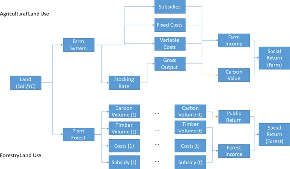
**Figure 1.** Structure of the Forestry Land use Change Microsimulation Model

As State approval is required both to plant forests and to harvest timber, with a legal requirement to replant following harvesting, and given the difficulties in returning forest-land to pasture or tillage, this analysis models a permanent land use change from agriculture to forest. Starting at the top panel of figure 1, the characteristics of the private and social return to agricultural uses are described. Different environmental characteristics are optimal for different farm systems (dairy, cattle, sheep, tillage etc.). However, the return to each of these systems is quite different. Similarly, the environmental footprint in relation to carbon emissions from animals (methane) and pasture or crops (nitrous oxide emissions from fertiliser and nutrient application) and greenhouse gas emissions from other inputs such as energy are quite different, depending on the farm system, the nature of production and the level of intensity and efficiency on individual farm systems. Given this heterogeneity, the starting position for the model is the nationally representative distribution of Irish farms in the Teagasc National Farm Survey (NFS),² which captures most of the diversity of farms. Subsidies vary by policy intervention, farm size, location of the farm and historical production levels. A carbon emissions model is employed to simulate the carbon emissions from each of these farms. For most crops, the production cycle is annual, as crops are planted and harvested annually, or follow an annual growth curve in the case of permanent pasture. As a result, the NFS uses an annual accounting framework.

However, forests have longer growth cycles than agriculture, spanning from tree planting to maturity and potential harvesting. The length of this cycle depends on the environmental context, productivity or yield class, tree species and the management regime of the forest in terms of thinning and harvesting. As the volume of timber increases over time, so too does the carbon stored or sequestered (described later in more detail). As planting, thinning and harvesting tend to be undertaken by contractors rather than foresters, there is not as much heterogeneity in management efficiency between forests as there is between farms. As in the case of agriculture, forest incomes depend to a considerable degree on subsidies.

The incorporation of carbon sequestration in a microsimulation model is challenging in relation to the assumptions used. A criticism of the literature is that there is quite a wide variety of assumptions used in carbon calculations (Asada et al., 2020), which can have a considerable impact on the results. Additionally, these assumptions are often poorly documented. This paper sets out to document the data sources, coefficients, assumptions and model validations of a microsimulation of a land use change to substitute an agricultural enterprise with a forest as is commonly incentivised in Western European countries such as Ireland, UK and Belgium. In this analysis, we use Irish data and coefficients. All modelling is undertaken using STATA.

Microsimulation modelling of private and social income requires the estimation of the following components:

Forest income is comprised of both afforestation subsidies and market income arising from timber sales as a function of the characteristics of different land types and alternative land uses. The estimation of timber sales requires forest growth data as a component of a forest bio-economic model of costs and market income.
Farm micro-data are necessary to estimate the agricultural market and subsidy income foregone on planting in order to model the carbon emissions of different farms.
Quantification of the sequestration of forest carbon and the agricultural emissions displaced from the superseded enterprise, dependent on soil variability and the superseded agricultural enterprise.
Future valuation of carbon.

2.1. Private (financial) impact of farm afforestation

Afforestation involves an upfront investment with a long time-frame before a return is realised. In order to compare the returns from forestry with annual returns from agriculture, a net present value (NPV) (Pingoud and Wagner, 2006) life-cycle framework is necessary. As the planting of former farmland also incurs an opportunity cost ,the NPV of Net Private Forest Income is modelled as private forest income less agricultural income foregone on a per hectare basis, varying by land and farm conditions where:

and where fixed forest costs include annual insurance, maintenance and roadways. Forest establishment costs are also included (but are partially offset by planting grants (subsidies).

Agricultural net market income or net margin is defined similarly by Hennessy et al., 2013 as:

A g r i c u l t u r a l N e t M a r k e t I n c o m e = O u t p u t V a l u e - V a r i a b l e C o s t s - A g r i c u l t u r a l F i x e d C o s t s

As afforestation generally takes place on a small proportion of land within a farm (DAFM, 2015), farmers continue to incur fixed agricultural (sunk) costs such as depreciation, buildings, machinery, land improvements and interest repayments on loans or ground rents after planting. Because these sunk costs generally remain unchanged, for simplicity purposes fixed costs are not included in the equations. Instead, a variable costs and income approach to calculating farm income (market gross margin) is adopted:

A g r i c u l t u r a l N e t M a r k e t I n c o m e = O u t p u t - V a r i a b l e C o s t s

In addition to direct costs that are incurred in forest establishment, management and harvesting, there are indirect opportunity costs associated with no longer being able to use the land for agriculture, namely the loss of annual agricultural income. This is accounted for by including the agricultural income foregone as an annual cost for each year of the forest rotation.

2.2. The Public Good (carbon) Impact of Farm Afforestation

There are three components of the public good impact: forest carbon storage (sequestration), displacement of agricultural GHG emissions from the planted land and the valuation of the sequestered/emitted carbon.

Six carbon pools contribute to gains (carbon sequestered) and losses (to the atmosphere) in different ways, with each varying by the soil attributes of the land on which planting occurs:

There is a slow increase in soil organic carbon (SOC) in mineral soils over time, whereas organic (peat) soils lose carbon on drainage and planting
Carbon is stored incrementally in forest biomass over time, (depending on the tree species planted and on the soil and climatic conditions of the planted land) in:
- above ground biomass (>7cm) and
- below -ground biomass (roots >5cm), until the wood is either harvested (removed), decomposes or is combusted.

Decomposing material such as
- dead organic matter (DOM) litter (decaying needles/leaves, branches <7cm diameter) and
- wood from dead trees (above/below ground >7cm) can decompose and add to SOC over time
Wood removed as harvested wood products (HWP) (products in current use from domestic harvests) continue to store carbon until they either decompose (rot) or are combusted.⁴ The half-life of the carbon stored depends importantly on the nature of the harvested wood products and on the disposal and decay rate at end of life for the wood products.

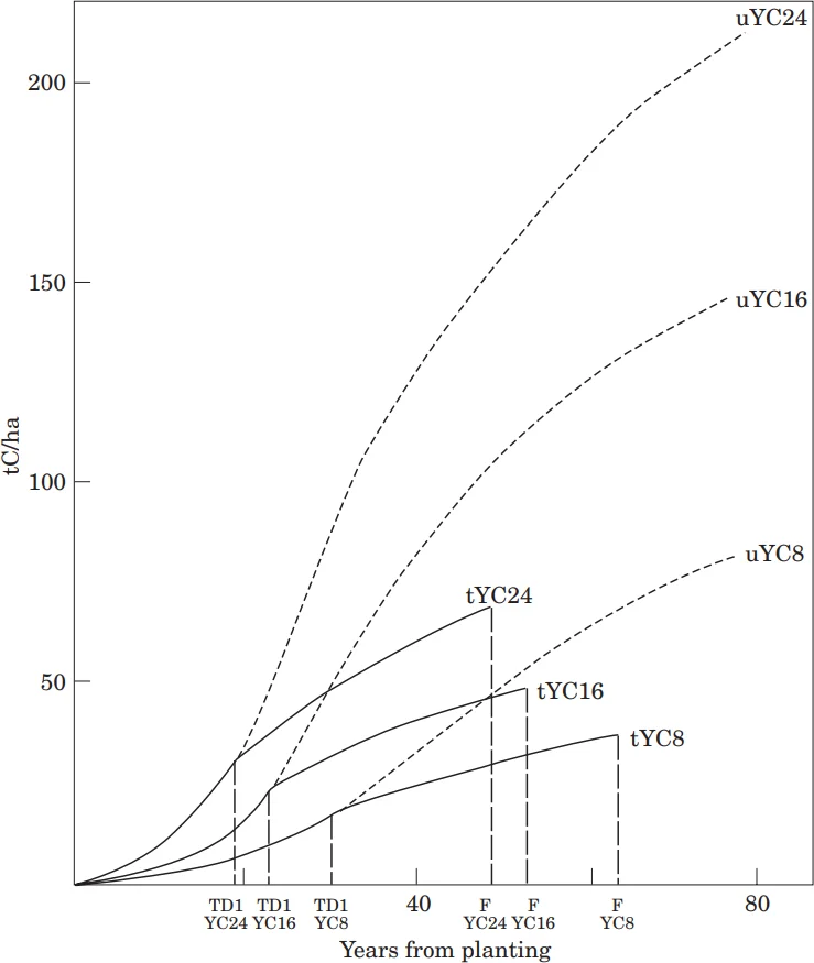
A visualisation of total carbon storage over time is presented for these pools for thinned and unthinned forests and for a range of forest yield classes in Figure 2. Yield Class is a measure of forest site productivity and is reported as the average annual timber production over the life-cycle of a forest measured in cubic metres per hectare per year ( $Missing \left or extra \right$ ).

**Figure 2.** Total carbon (C) storage curves for unthinned (u) and thinned (t) Sitka spruce yield class 8, 16 and 24

The agricultural GHGs displaced on planting are (a) methane $(C H_{4})$ emissions from enteric fermentation in ruminant animals and manure management, (b) direct and indirect nitrous oxide( $N_{2} O$ ) emissions for each livestock sector i.e. manure management, fertiliser application and dung/urine deposition, along with fertiliser emissions from tillage. Carbon dioxide ( $C O_{2}$ ) emissions from fuel and electricity are included for both agriculture and forestry.

The final component of estimating the public good return to farm afforestation is the application of a carbon value to the carbon sequestered/emitted. The concept of the social cost of carbon (SCC) relates to the economic cost caused by an additional tonne of carbon (or equivalent) emissions (Nordhaus, 2014). The cost of additional $C O_{2}$ in the atmosphere varies with the level of GHG emissions and as a result, Smith and Braathen (2015) highlight specific assumptions that need definition with regard to SCC and the current and future levels of GHG concentrations, against which its effects are to be measured. The SCC estimates the monetary value of the incremental impact of an additional tonne of emissions. Abstracting from the complexity of these elements of the SCC and from tax, regulation and inconsistent assumptions across sectors, the SCC would equal the carbon price, i.e. the marginal cost of emissions reduction (the present value of the damage caused per unit of emissions) (Nordhaus, 2014).

There is significant variation within the literature with regard to the social value of carbon (NESC, 2018), both in terms of the discount rate and the price of carbon. Stern (2007) valued carbon at $85 / $t C O_{2}$ . A report from the Interagency Working Group (IWG) on Social Cost of greenhouse gases estimated a carbon price of between $36 and $42 per $t C O_{2}$ in 2007, using a 3% discount rate (IWG, 2013). On the other hand, (Moore and Diaz, 2015) attribute a lower discount rate as a result of damages caused by climate change and report a SCC value of $220 per tonne of additional $C O_{2}$ (Moore and Diaz, 2015). While the Irish conventional discount rate for forest investments is 5% (Clinch, 1999), this paper includes scenario analysis of the impact of a range of discount rates on the carbon value.

As one of the rationales for this analysis is the examination of the social return to the land use change from agriculture to forestry as a mitigation measure for agricultural GHG emissions, we require an indication of the substitution effect in physical terms. For this purpose, we utilise the carbon value recommended by the Irish government as the shadow price of carbon for non-ETS sectors. Given the uncertainty around carbon valuation, we utilise the shadow prices for different years i.e. 2019 (€20), 2020 (€32), 2030 (€100), 2040 (€163) (DPER, 2019).

In estimating the social return to land use change, the value of forest carbon sequestered and GHGs emitted by agriculture and the relative private returns are included as follows:

\begin{aligned} (9) & N P V S o c i a l I n c o m e_{A f f o r e s t a t i o n o f a g r i c u l t u r a l l a n d} & = N e t P r i v a t e F o r e s t I n c o m e - \\ (10) & A g r i c u l t u r a l N e t M a r k e t I n c o m e + \\ (11) & V a l u e o f N e t C a r b o n S e q u e s t e r e d b y F o r e s t s \\ (12) & + V a l u e o f G H G s E m i t t e d b y D i s p l a c e d A g r i c u l t u r e \end{aligned}

In order to compare (a) forest returns over different rotation lengths and (b) annual agricultural returns with long-term forest NPVs, an annual equivalised of NPV is required (Herbohn et al., 2013).⁵

3. Methodology

3.1. C-ForBES Microsimulation Framework⁶

Microsimulation techniques are increasingly used to deal with the complexity of cross-system and cross-country agricultural analyses ( Thorne and Fingleton, 2006) and for analyses requiring the use of counterfactual data (O’Donoghue, 2017). The generation of forest and agricultural income and carbon streams in this analysis builds on the farm afforestation microsimulation framework developed by Ryan and O’Donoghue (2019), and the ForBES (Forest Bio-Eeconomic system model) Ryan et al. (2018) by including a carbon sub-model to estimate forest and agricultural carbon, namely the (carbon) C-ForBES model.

C-ForBES first estimates the private forest income streams associated with planting one hectare of SS forest in 2015, for the land types represented by the Teagasc NFS soil codes. In modelling the replacement of a hectare of an agricultural enterprise with one hectare of forest, a mechanism is necessary to relate the productive potential and physical constraints of individual farms to their forestry potential. This is achieved as described in Ryan et al. (2018) using a classification developed by Farrelly (2011), that assigns Sitka spruce Yield Classes (YC) to the Teagasc NFS Soil Code (SC) used to represent the dominant soil class in the NFS. Using this classification, the mosty productive YC 24 is associated with the (best) farm soils (SC1) that are suitable for a wide range of uses, while the most limiting farm soils (SC6) equate to the lowest yield class (SS YC 14).

Annual agricultural private returns are derived using the Teagasc NFS 2015 dataset, which is nationally representative by system and size. C-ForBES incorporates this income foregone as a cost, which is held constant in each year of the forest rotation. A discount rate of 5% is used to generate the NPV of private income streams, which are presented in terms of annual equivalised (AE) NPV of income (as annual equivalised NPV may not be equal to an average over time). In the next stage, agricultural GHG emissions, (methane $(C H_{4})$ nitrous oxide ( $N_{2} O$ ) and carbon dioxide ( $C O_{2}$ ) are estimated at individual farm level.

3.2. C-ForBES Agricultural GHG emissions estimation

In order to estimate the emissions per hectare, the average livestock density per hectare (taking soil code into account), is calculated using methodologies consistent with the Teagasc NFS. Displaced agricultural emissions are calculated for tillage and for each of the livestock systems (dairy, cattle and sheep) on a per animal basis (taking soil code into account). Per hectare livestock emissions are derived using Teagasc NFS methodologies and animal numbers and age categories from the 2015 Teagasc NFS, providing livestock equivalent units (LU) per ha (one dairy cow equals 1 LU $h a^{- 1}$ ). NIR (2018) system-specific emission factors (EF) for methane ( $C H_{4}$ ) and $N_{2} O$ emissions for tillage, livestock grazing and manure management practices, fertiliser inputs and fuel and electricity usage are then applied. Tables A2; A3 (Appendix 1) present the agricultural activity data by farm system and soil code and Table B1 presents the 2015 emission factors from the common Reporting Framework used by the EPA National Inventory Reports. Methane and nitrous oxide are converted to carbon dioxide equivalent CO ₂ e (a measure used to compare the emissions from various greenhouse gases on the basis of their global-warming potential (GWP) where the GWP for methane is 25 and for nitrous oxide 298) and the results are presented in Table 1.

Table 1. Agricultural Carbon Emission Factors and GHG equivalent conversions

	Energy CO ₂	Energy CH ₄	Energy CH ₄	CH ₄	Agri CH ₄	Total CO ₂	Total CO ₂e
	tCO ₂/€	tCH ₄/€	tCO ₂e/€	tCH ₄/head/yr	tCH ₄/head/yr	tCO ₂e/head	tCO ₂e/LU
Dairy				0.124	0.00012	3.129	3.129
Cattle				0.051	0.00013	1.308	2.975
Sheep				0.006	0.00001	0.152	0.684
Horses				0.020	0.00015	0.544	1.238
Pigs				0.006	0.00003	0.262	1.176
Poultry				0.000	0.000001	0.00590	0.006
Fuel	0.003	0.00000154	0.00000015
Fertiliser					0.000032
Crops					0.00000041
CO ₂ equiv conversion factor	1	25	298	25	298

Source: Common Reporting Framework 2015^[6]

Next, C-ForBES estimates carbon in forest soils, live biomass, dead organic matter and harvested wood product pools. As carbon gains and losses can vary considerably depending on forest management practices, for transparency purposes, this analysis documents all relevant assumptions and equations in Table B1 (Appendix B) (denoted by [ ]). Forest management assumptions [1] are those used in the ForBES model and based on the Teagasc FIVE (Forest Valuation and Investment Evaluator) (see Ryan et al., 2016). Forest subsidies [2] are provided by the ForSubs model (Ryan et al., 2014). Timber volumes are derived using the merchantable timber volume (MTV) from the Edwards and Christie (1981) yield models for relevant yield classes. Establishment and reforestation costs [3] are derived from Teagasc FIVE. Roundwood from thinnings and final harvest is assumed to be sold standing and income projections are derived using MTV and published timber prices [4].⁷ Several validations and sensitivity analyses and undertaken. In estimating the social value of carbon, C-ForBES replaces the afforestation subsidy with a carbon subsidy, based on carbon values in future periods. Finally, environmental consequences of farm afforestation are examined, namely the magnitude of the substitution effect of replacing one hectare of livestock (and the associated emissions) with one hectare of trees.

3.3. C-ForBES Forest Carbon Estimation

For UNFCCC reporting purposes, Ireland adopts a long-term gains and losses approach in National Inventory Reports (NIR) based on forest and agriculture activity data supplied by government agencies, where national carbon stock changes (CSC) over time are reported annually for all sectors nationally. In this study however, the focus is on the net carbon implications of a land use change from agriculture to forestry where future values and costs are discounted to a given year (2015) on a per hectare basis. Where possible and/or feasible, the study utilises the relevant forest and agriculture emission/sequestration factors using the information provided in NIR. Taking the long-term nature of carbon losses and gains into account, this analysis is undertaken for a 200 year period.

Noting the considerable variability in the literature in relation to the parameters and assumptions used for forest carbon estimation, sensitivity analysis of the variability in some of these parameters was undertaken. We reference the assumptions and carbon emission/sequestration factors used in this analysis in the Appendix, along with differing assumptions as used in two particularly relevant but diverse analyses: the Bateman and Lovett (2000) paper - an economic and GIS analysis of the valuation of carbon sequestered by Sitka spruce and Beech in Wales and the Irish National Inventory Report (NIR, 2018) - the national accounts framework for GHG emissions reporting (1990-2016) to the United Nations Framework Convention on Climate Change (UNFCCC). Forest carbon is thus estimated for each of the six carbon pools.

According to Wellock et al. (2011) there is little change in soil organic carbon (SOC) following planting of forests on (formerly grassland) mineral soils, although there is a gradual build-up of carbon over time. Afforestation on organic soils on the other hand, can result in significant emissions (Byrne and Farrell, 2005) that are influenced by water table, soil depth and weather. In reviewing the literature however, values for carbon change in soils vary considerably in different analyses. The soil carbon emissions factor (EF) has increased over successive Irish NIRs, but are lower than those assumed by Bateman and Lovett (2000, p. 316). While considerable historic planting was undertaken on organic soils in Ireland, current forest policy limits afforestation on peats in environmentally sensitive areas. As there are insufficient data in the Teagasc NFS in relation to the soil composition of individual farms, this analysis makes the simplifying assumption of planting on mineral soils only. However, a sensitivity analysis of planting on peats is included (Table 2) using the NIR (2018) EF for peats [6].

Table 2. Private Returns to Planting SS Forest in 2015 (annual equivalised (AE) of Average NPV per ha) at 5% discount rate

Yield Class	Average AE of NPV (€ $h a^{- 1}$ )
24	563
20	473
18	425
14	355

Source: C-ForBES

Carbon Models, Assumptions and Validation

This section describes the carbon storage per hectare in SS forest livewood biomass (both above and below ground), which is estimated where possible using country specific parameters from the 2018 NIR for yield classes 14-24. Total carbon stock (C) is estimated over successive forest rotations from equation 1:

(1)

C = \sum_{i = 1}^{n} {V_{i} \cdot D_{i} \cdot B E F_{i} \cdot C F} \cdot P

First, the MTV per hectare (denoted by V_i) is derived from the Edwards and Christie (1981) forest yield models. However as these models don’t include early annual growth rates, a sigmoid function is utilised to interpolate growth up to the age of first thinning [7]. The carbon mass of live biomass is calculated is the product of volume (MTV), wood density [8] (ratio of oven dry weight of timber to green volume ( $D_{i}$ ) and carbon fraction ( $Missing \left or extra \right$ ) [9] ,which is generally about 50% of wood biomass) (Dewar and Cannell, 1992).

The dynamic BEFs [10] used in the NIR (2015), derived from research conducted by Black et al. (2004) are used in this analysis. However a sensitivity analysis using both static and dynamic BEFs is also undertaken (Table 3). P [11] is the productive forest area.

Table 3. Average Private Returns (Gross Margin € ha ⁻¹) to Agriculture by Soil Code and Farm System (2015)

SC	YC	Specialist Dairy	Cattle Rearing	Cattle Other	Sheep	Tillage
1	24	1566	1029	996	954	1098
2	24	1181	855	882	1066	1186
3	20	1145	766	764	740	1103
4	20	1082	656	878	859	803
5	18	670	497	550	471
6	14	584	583	356	681
All	All	1237	784	867	811	1114

Source: Teagasc NFS (2015)

Note: SC: Teagasc NFS Soil Code (1 – Best, 6 – Worst), YC: Forest Yield Class

As only a proportion of carbon from the above ground part of the tree is used in harvested wood products, we divide total carbon between above ground $C_{A G}$ and below ground $C_{B G}$ :

(2)

C = C_{A G} + C_{B G}

The share of the below ground carbon is defined by the root ratio parameter (denoted by $R$ ). In general, broadleaf species have a larger root mass than conifers (Morison et al., 2012). This analysis uses the NIR (2015, 2018); country specific ratio for SS [12] (Black et al., 2009).

The estimation of live biomass carbon relates to above ground biomass:

(3)

V_{E C, i} = V_{i} \cdot (1 - R)

Therefore, we use an adjusted version of the carbon equation to differentiate above ground (equation 4):

(4)

C_{A G} = \sum_{i = 1}^{n} {V_{E C, i} \cdot D_{i} \cdot B E F_{i} \cdot C F} \cdot P

and below ground carbon stocks (equation 5):

(5)

C_{B G} = \sum_{i = 1}^{n} {\frac{V_{E C, i}}{(1 - R)} \cdot R \cdot D_{i} \cdot B E F_{i} \cdot C F} \cdot P

The DOM (dead organic matter) pool is comprised of litter and deadwood. Litter [13] is modelled according to algorithms outlined in NIR (2018) and represents the transfer of carbon from the above ground pool to the litter pool, based on the leaf/needle biomass and the foliage turnover rates (6.7 years for conifers and annually for broadleaves (Tobin and Nieuwenhuis, 2007). Litter is assumed to decompose at a rate of 14% per year (NIR, 2018-p 222).

The carbon inputs to the deadwood [14] component of DOM in NIR (2018) DOM in NIR (2018) include tree mortality, tree roots and harvest losses. We follow the assumptions of Black (2016) of a tree mortality rate of 1.6% of volume per year, with dead trees decomposing at the same rate as deadwood i.e. 14% per annum.⁸ Although beyond the scope of this analysis, the NIR reports the gradual accumulation of DOM, which can be an important component of carbon stock change over long time horizons.

Carbon is also transferred between DOM pools through complex mechanisms including decay, transfer and disturbance, however, these transfers are beyond the scope of this analysis.

At the point of thinning or final harvest $H_{i}$ , harvest losses (waste) $L_{i}$ [15] are incurred and are assumed to be oxidised. These losses can be significant, particularly at first thinning and it is important to adequately take account of these losses to the system (Ryan et al., 2016). The above ground biomass $C_{A U}$ remaining on the site and available for removal from the forest therefore is:

(6)

C_{A U} = C_{A G} \cdot (1 - L_{i}) = \sum_{i = 1}^{n} \begin{matrix} {V_{E C, i} \cdot D_{i} \cdot B E F_{i} \cdot C F} \cdot P \cdot (1 - L_{i}) \end{matrix}

Energy wood is considered to be immediately oxidised to the atmosphere [16] and accounts for a significant proportion (34%) of the biomass C removed from forests, according to the Knaggs and O’Driscoll (2017) ‘Wood Flow’ report.

A significant amount of non-forest carbon is stored in harvested wood products (HWP) for differing lengths of time, depending largely on the end-use and its half-life (IPCC, 2006). The inflow to HWP employed here is modelled as:

(7)

I n f l o w = C_{A U} ∙ (1 - E_{i})

where $E_{i}$ represents wood energy losses. The proportions of sawnwood, wood-based panels and paper and paper-board making up the HWP on an annual per hectare basis are taken from NIR (2018) [17]. Saw-milling losses are taken into account on the basis of the Knaggs and O’Driscoll (2017) report [18]. In estimating the liberation of carbon from HWP we follow the method of Pingoud and Wagner (2006) which is used in NIR (2018) as follows:

(8)

{C H W P}_{j} (i + 1) = e^{- k} ∙ {C H W P}_{j} (i) + [\frac{(1 - e^{- k})}{k}] ∙ I n f l o w (i)

This analysis makes the simplifying assumption that all extractions from forests have the same share of final uses. It is likely however that a high proportion of early thinnings are used for energy, while wood from later thinnings and clearfell is more likely to be used for longer half-life HWP such as sawn-wood and wood-based panels. More comprehensive and further research would be required to disaggregate these allocations, however, sensitivity analyses of different value chain assumptions are undertaken in Appendix 3.

Combining the carbon pools, total forest carbon stock is expressed as tCO ₂ ha^-1 yr^-1 (using IPCC conversion factors [19]) to be comparable with agricultural emission metrics.

4. Data and Summary Statistics

The primary data source in this paper is the Teagasc NFS, which collects detailed information from a representative sample of farms and is Ireland’s input to the EU Farm Accountancy Data Network (FADN). Using data for 2015, agricultural cost and revenue streams are generated for each of six agricultural systems (dairy, cattle rearing, cattle other, sheep, tillage and mixed livestock) on six NFS soil codes.⁹ C-ForBES links these agricultural data with the forest yield classes (Edwards and Christie, 1981) using the classification described earlier and forest management costs and revenues in Teagasc FIVE (Teagasc, 2012). Table 3 describes the average agricultural gross margin (including subsidies) per hectare for the livestock farm systems by soil type and corresponding yield class. There is a broad correlation between soil code and the gross margin per hectare as the highest gross margins are achieved on dairy and tillage farming (particularly on the less limiting soil codes), while cattle and sheep farming have lower gross margins per hectare.

Table 2 reports the average return per hectare from planting Sitka spruce (SS) for a range of yield classes, reflecting the opportunity cost of agricultural income foregone. The impact of better quality land as represented by high yield class is clearly evident.

4.1. Carbon Models, Assumptions and Validation

The calculation of carbon sequestration in forests is sensitive to the data, yield model and forest management assumptions used. A range of methodological assumptions used in different carbon modelling approaches is examined as part of this study and presented in Appendix C, showing variability in above and below ground carbon sequestration biomass inputs and carbon liberation from HWP and the magnitude of carbon losses from harvesting and from energy wood. Such variability (particularly in relation to losses from harvesting and wood energy and the impact on long-term sequestration in HWP) has considerable impacts on carbon sequestration and loss, with consequent impacts on the social value and the net carbon impact of the land use change from agriculture to forestry. In order to provide clarity and transparency in the modelling approach utilised in this study, all forest management assumptions, information on parameters such as productive forest area, species, species mix, rotation length, allocation of timber to different end-uses and other practical aspects of forest management are documented in Table B1 (Appendix B).

5. Results and Discussion

In this section, the results of the carbon sequestration analysis and are presented and discussed in the context of the modelling assumptions used for forest carbon pools and validation against other analyses. For simplicity purposes, ‘No Thin’ scenarios are presented, unless stated otherwise. Next we present the private and social returns to the land use change with sensitivity analyses around the parameters used and lastly, the distributional analysis is presented.

5.1. Carbon Sequestration

First, we illustrate the accumulation and loss of carbon over a 200 year period for Sitka spruce yield class 18 (no thin) in Figure 3. The largest increase in carbon is evident in the above ground livewood, particularly in the early years, with an acute loss of carbon at the point of harvesting, when timber is removed from the forest. The lower rate of sequestration in the below ground livewood reflects the 80/20 above/below ground ratio.

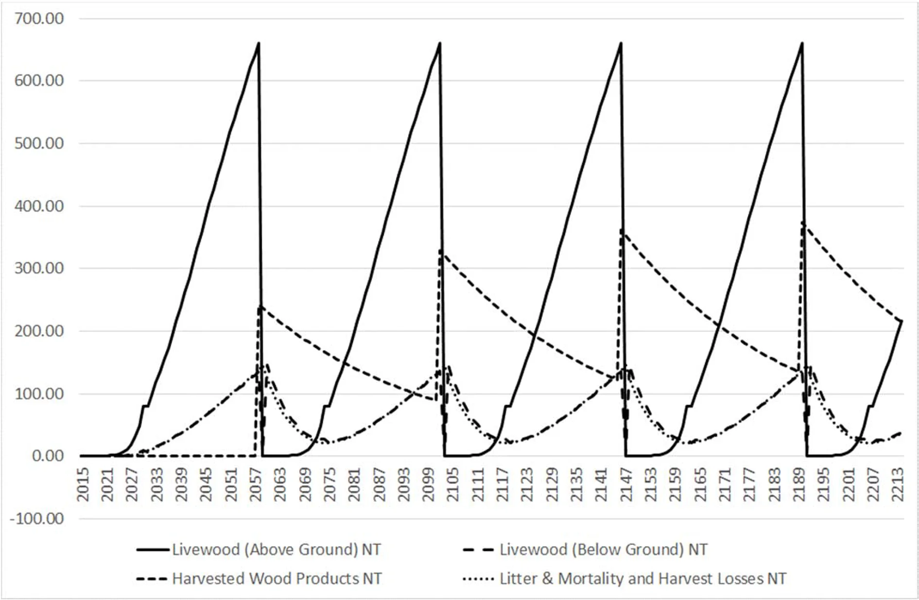
**Figure 3.** Carbon (C) Sequestration/Loss for No Thin (NT) Yield Class 18 over 200 years

At clearfell (final harvest), the above ground biomass declines to zero, while the below ground biomass transfers slowly to the DOM pool. There is an immediate decline in carbon in HWP at harvest, relative to above ground livewood, as just over a third of the livewood is used for energy (Knaggs and O’Driscoll, 2017) and is immediately oxidised. Harvesting (roundwood) losses are also incurred during the harvesting process.

In contrast to the no thin scenario presented in Figure 3, on thinning (periodic removal of trees), there is an initial drop in above ground biomass, followed by a subsequent increase in growth (and carbon sequestration) due to the greater availability of light, moisture and nutrients for the remaining trees. As each thinning occurs, livewood carbon declines and the cumulative carbon in HWP increases, albeit declining if the biomass is combusted (oxidised). An important difference between thinned and unthinned forests is that harvest losses at thinning can be substantial, particularly in the case of first thinning.

5.2. Private and Social Returns to Land use Change from Agriculture to Forestry

In this section we examine both the private and the social (private + public) return to farm afforestation. In order to model the social impact of land use change, it is necessary to include the alternative land use, namely agriculture, and to combine the private economic components with the public component. The definition of social return can be quite broad incorporating all monetary and non-monetary aspects, whereas the private return to a landowner represents only the life-cycle monetary impact of moving from agriculture to forestry. However this clearly ignores significant public good impacts in relation to carbon sequestration. There are of course other aspects of the return, including the private return to other value chain actors such as timber mills and other ecosystem services such as biodiversity or water quality. To keep the analysis tractable but useful, we adopt a narrower definition of social return to a land use change, i.e. the combination of the private return to the landowner plus the value of the net carbon sequestration of the land use change.¹

Table 4 describes the economic dimension of planting one hectare of forestry. Columns A, B, C and D respectively report market gross margin (MGM) and direct payments/subsidies for agriculture, forest MGM and forest subsidies. As expected, MGM for agriculture and forestry is correlated with soil type, while agricultural subsidies have a redistributive focus and are uncorrelated with soil type. Forest subsidies are paid as compensation for loss of agricultural income and as an implicit incentive for the provision of forest ecosystem services and are also uncorrelated with soil type.

Table 4. Economic Components of Agriculture and Forestry (2015) (Annual Equivalised NPV per ha (€)

Soil Code	Agriculture		Forestry
	Mkt Gross Margin /ha (A)	Subisides /ha (B)	Mkt Gross Margin /ha (©)	Subsidies /ha (D)
	€	€	€	€
SC1/YC24	1200	366	224	306
SC2/YC22	792	388	224	306
SC3/YC20	803	342	154	302
SC4/YC18	731	351	154	302
SC5/YC16	356	314	124	300
SC6/YC14	258	326	52	298
Average	878	359	155	296

The carbon sequestration/emissions resulting from planting one hectare of SS forest replacing agricultural enterprises, are calculated by applying the carbon dioxide equivalent coefficients per hectare from Table 1 to farm-level activity data (both direct and indirect emissions) and forest life-cycle (200 years) data. In facilitating comparisons between agriculture and forestry, life-cycle sequestration from forestry and emissions from agriculture are annualised using a 5% discount factor to produce the average discounted tonnes of carbon dioxide equivalent per hectare $(t C O_{2} e) h a^{- 1}$ for the farm systems and soil types. These are reported as average annual equivalised values in Table 5 (columns E and F). The components that result in these returns are also reported, showing that for higher quality soil types, the quantity of carbon sequestered per hectare is almost twice that of the animal emissions displaced. For SC5, the ratio is closer to a factor of three. The implication here is that replacing agriculture with forestry on the best land would result in a reduction of net carbon dioxide emissions of 24.1 tCO₂e on average over the life-cycle. In terms of the corollary (replacing agriculture on poorer soils with forestry), the net reduction or sequestration is lower, because of (a) the lower carbon sequestration from forests and (b) because the substituted enterprise had lower emissions.

Table 5. Average Annual Equivalised Social Return to Planting one hectare of Unthinned Forest (2015) Displacing Agriculture

Soil Code	Private Return¹⁰	Agriculture	Forestry	Social Return
	(C+D) – (A+B) (€/ha)	E¹¹	F¹²	C – (A+B) + (F-E)*P¹³ (€/ha)
tCO ₂ Value (P)	€0	tCO ₂	tCO ₂	€20	€32	€100	€163
SC1	1036	-9.2	14.9	-556	-268	1365	2878
SC2	651	-8.4	14.9	-185	95	1680	3148
SC3	690	-7.5	11.8	-304	-72	1239	2455
SC4	627	-7.4	11.8	-242	-11	1298	2511
SC5	246	-4.5	10.8	59	242	1281	2243
SC6	234	-4.9	7.8	19	171	1031	1828
Total		-8.0	13.4	-359	-103	1347	2691

Note: No-thinning assumed; BEF Factors from the 2015/18 National Inventory Reports are used;

All values are discounted using a 5% discount rate. Sensitivity Analyses

However, we would also like to examine the impact of taking carbon into account in the returns to planting. In generating the social return to planting, as the afforestation subsidy (D) is not a direct measure, it is replaced with a carbon subsidy (carbon emissions (agriculture E and forestry F) x Cost per tCO ₂, for a range of carbon values. There is not currently a carbon instrument in place, (as the inclusion of carbon in incentives could act as a negative driver if farm forest owners were fined for carbon losses to the atmosphere on harvesting), thus the more pragmatic solution is to provide an indirect subsidy at planting and tax-free incentives for timber sales. Therefore as we not modelling a behavioural response, static carbon values are included.

Table 5 reports the average private and social returns from the afforestation of one hectare of agricultural land and shows that on average, the private return to forestry is lower than the return from agriculture in the current policy environment, but becomes increasingly positive when increasing carbon values are substituted for afforestation premium. At low values of €20 and €32, (similar to the lower bound carbon price in the national agricultural GHG Marginal Abatement Cost (MAC) curve (Black et al., 2004) of €25 per tonne of CO ₂, the social return for planting a hectare of forest exceeds that of agriculture on the poorest soils. Once the carbon value is increased to €100 and €163 (reflecting the Irish government shadow price of carbon for 2030 and 2040 respectively) all soil codes have a higher social return from forestry than from agriculture, with the highest returns on the most productive soils. All values are discounted using a 5% discount rate

5.3. Sensitivity Analyses

The analysis undertaken here assumes the same allocation of wood to the value chain from thinnings and from final harvest; in other words, the share of wood uses allocated to energy, sawn wood and wood-based panels is consistent across thinnings and final harvest. Actual allocations can vary considerably, depending on management regime, market conditions and proximity to wood energy and sawnwood processors. In reality, a large proportion of early thinnings is likely to be used for wood energy, with the proportion allocated to sawnwood increasing as tree size increases. However there are no data sources for these allocations, therefore, we would like to test the impact of allocating all thinnings to wood energy.

In Table 6, the impact of different assumptions re the allocation of thinnings to either wood products or energy are presented for two extreme assumptions: (a) all harvested wood (thinnings and clearfell) is allocated proportionally to energy and to harvested wood products and (b) all thinnings are allocated to energy and immediately combusted. These assumptions can be regarded as an upper and a lower bound. We see that when all thinnings are used for energy, the amount of clearfell wood used for energy decreases by about 40%. The annual equivalised total tCO ₂ is about 11% higher for the original assumption, reflecting greater earlier storage than when all thinnings are used for energy. If the values were undiscounted, there would be no difference, as the same amount of wood is burnt for energy under both scenarios. In order to get a more precise estimate, a more detailed evaluation of different wood flows over different parts of the life-cycle would be required.

Table 6. Comparing the Annual Equivalised tCO ₂ for Thinned Forests by Soil Type if all thinnings are used for energy

Soil Code	Equal Allocation from Thinnings and Clearfell to Energy	Thinnings only Allocated to Energy
1	10.77	9.60
2	10.77	9.60
3	9.04	8.16
4	9.04	8.16
5	9.14	8.37
6	5.37	4.83
Average	9.98	8.95

Note: 2015/18 National Inventory Report Assumptions

The impact of the land use change from agriculture to forestry is at the core of this analysis. While afforestation on blanket peats is no longer grant-aided, many farms have areas of peaty (organo-mineral) soils. However, the available farm-level data are insufficient to distinguish between peaty and minerals soils. C-ForBEs assumes that the SS forest is planted on mineral soils, however we are interested in the sensitivity of planting on peat and mineral farmland. Table 7 highlights the lower carbon sequestration on peats by about 2tCO ₂ per ha, given soil carbon losses at the time of planting due to drainage on peaty soils.

Table 7. Total Annual Equivalised tCO ₂ Forest Carbon Sequestration for Mineral and Peat Soils by Yield Class

Yield Class	Mineral	Peat
24	12.69	10.56
24	12.69	10.56
20	10.44	8.32
20	10.44	8.32
18	9.34	7.21
14	7.60	5.48
Average	11.56	9.43

Note: For simplicity purposes in peat calculations, these values are calculated using EFs from NIR (2012)

The use of market price for timber and carbon values can also lead to different conclusions. The market prices used in this study are based on ten year relatively stable average prices [4], while the carbon values used are the official national policy, setting out carbon prices [20] for the next 20 years. In order to account for this risk, analysts use higher discount rates where risk is considered to be super-normal. Thus the discount rate can have a considerable impact on the social return to planting. The analysis thus far assumes a 5% discount rate. Table 8 highlights how small changes (at different carbon values) can have large impacts on the social return. The share of farms where the social return is higher for forestry increases with carbon value and for lower discount rates. At a carbon value of €32 and 4% discount rate, 82% of farms on average have a higher social return from forestry. As the discount rate increases, the share of farms that have a higher social return from forestry falls, but remains above 70% even at 7% discount rate. For lower discount rates, the proportion is higher for almost all farms.

Table 8. Share of Farms with greater social returns from Forestry than from Agriculture (Annual Equivalised NPV-2015) for a range of Discount Rates

Discount Rate	0	1	2	3	4	5	6	7
Carbon Value (€):	32
Soil Code
1	1.000	0.998	0.958	0.846	0.720	0.643	0.597	0.563
2	1.000	1.000	0.991	0.940	0.923	0.895	0.853	0.824
3	1.000	1.000	0.955	0.868	0.805	0.755	0.736	0.724
4	1.000	1.000	0.969	0.922	0.844	0.814	0.779	0.741
5	1.000	1.000	0.979	0.932	0.919	0.912	0.912	0.903
6	1.000	1.000	1.000	1.000	1.000	1.000	1.000	1.000
Total	1.000	0.999	0.969	0.892	0.820	0.774	0.739	0.712

Distribution of Private and Social Returns

5.4. Distribution of Private and Social Returns

This paper thus far describes average carbon figures for different soils and sectors. However, these averages mask a wide distribution.Next we look at the distribution of farms, with Table 9 presenting distributional assumptions in relation to private returns and social returns. On average 32.4% of farms have positive private returns to planting, including forest subsidies. Replacing the afforestation subsidy with low carbon (subsidies) values of €20 and €32 per hectare, and using the most recent NIR (2015) assumptions for biomass expansion factors and also incorporating agricultural subsidies, the share of farms with a positive social return is 30.4% and 46.6% respectively. Using a carbon value of €100 per hectare, the share rises to 96.5%, while at a carbon value of €163 per ha, nearly all farms (99.9%) have positive social returns.

Table 9. Share of Farms with a positive Private and Social return to Forestry by BEF Assumption and inclusion of Forest Subsidy

	Private Return	Social Return
Carbon value (€)	0	20	32	100	163
BEF (NIR, 2012)
Incl Farm Subsidy	0.324	0.264	0.427	0.943	0.998
Excl Farm Subsidy	0.551	0.577	0.672	0.983	0.999
BEF (NIR, 2015)
Incl Farm Subsidy	0.324	0.304	0.466	0.965	0.999
Excl Farm Subsidy	0.551	0.594	0.697	0.991	0.999

Impact of substitution of trees for livestock

As a sensitivity analysis, we utilise earlier NIR assumptions (see also Table C2), finding an impact of about five percentage points for lower carbon values. We also test the sensitivity of whether afforestation occurs on land with or without agricultural subsidies, finding an unsurprisingly high impact.

5.5. Impact of substitution of trees for livestock - area of livestock emissions offset by a hectare of different types of afforestation

Farm afforestation is proposed as the largest potential mitigation measure for increasing livestock emissions in Ireland (Lanigan et al., 2019), thus we investigate the environmental impact of the land use change from agriculture to forestry by examining the livestock emissions that could be displaced by the carbon sequestered on one hectare of SS forest, measured in terms of land area (hectares of forest) and livestock emissions (LU per ha). For simplicity, results are reported in Table 10 for no thin (NT) forests for (a) planting a forest only - without accounting for the displaced livestock emissions from a land use change (No LUC), and (b) a land use change accounting for both forest carbon sequestration and the displacement of GHG emissions from agriculture.

Relating the livestock units per hectare (and the forest yield classes) across the soil codes, Table 10 represents the area (ha) of afforestation needed to offset emissions from livestock and reports that on average, the emissions from 1.68 hectares of land (with animals) are equivalent to the carbon sequestration from one hectare of (SS) forest (without land use change). When the displacement of livestock is taken into account, net sequestration increases to the equivalent of 2.68 hectares. This ratio increases with stocking rate, with a 25% gap between the highest and lowest soil codes, reflecting a strong correlation between animal stocking rate and tree growth, so the area is similar across all soil types, except soil class 5, although this may be due to lack of resolution of soil data at farm level. The corollary in terms of livestock units,¹⁴ is that one hectare of forestry displacing agriculture (with LUC), replaces 3.79 livestock units per hectare on average, with the number of livestock units displaced varying from 2.34 for the poorest soil types to 4.18 on the best soil types, and 2.38 LU per ha on average without LUC. Finally, we note that one hectare of thinned forest displaces fewer animal emissions than an unthinned forest, due to the lower sequestration associated with thinned forests. It should be noted also that this information relates to all land, including tillage. As tillage land is primarily used for animal feed, this is a reasonable assumption.

Table 10. Area of livestock production that could be offset by one hectare of SS, at different livestock densities (LUha⁻¹), with/without accounting for land use change (LUC) by soil code

Soil Code	Stocking Rate	Area (ha)offlivestock displaced by one ha of forest	Area (ha) of livestock displaced by one ha of forest	LU displaced per Ha of Forest	LU displaced per ha of Forest	LU per Ha of Forest
	LU per Ha	No LUC (not accounting for displaced emissions)	With LUC (accounting for displaced emissions)	No LUC	With LUC(No Thin)	With LUC (Thin)
1	1.57	1.62	2.62	2.56	4.13	3.03
2	1.52	1.76	2.76	2.67	4.18	3.03
3	1.33	1.59	2.59	2.12	3.45	2.69
4	1.36	1.59	2.59	2.17	3.52	2.75
5	0.87	2.38	3.38	2.06	2.93	2.29
6	0.90	1.61	2.61	1.44	2.34	1.85
Average	1.41	1.68	2.68	2.38	3.79	2.84

6. Conclusions

In this paper, we describe in detail the development of a microsimulation model to simulate the life-cycle impact of the incorporation of carbon emissions in the conversion of agricultural land to forestry, enabling the distribution of wider social returns to be modelled in addition to the private return. The paper is novel in that it brings together the literature on land use change, which focuses mainly on the social return to land at an aggregate spatial level, and farm level simulation analysis that focuses on private returns. Given the importance of afforestation as a driver of carbon sequestration and a mitigation measure for agricultural emissions, there is a policy imperative to combine both dimensions.

Reflecting the negative and positive externalities associated respectively with agriculture in terms of carbon emissions and with forestry in terms of carbon sequestration, the private returns for both land uses were modelled along with a measure of the value of the public good provision in terms of carbon sequestration. These reflect respectively the return from the market and the returns to society, accounting for carbon emissions and sequestration.

The analysis highlights that unthinned livewood is the largest forest carbon pool while the HWP pool is the largest non-forest pool and is perhaps where the greatest advances could be made in relation to the substitution of long-lived sawnwood products for concrete and steel, however the modelling of the substitution effect of replacing concrete and steel is beyond the farm level focus of this paper but is the subject of future work.It also highlights the influence of soil quality on forest carbon sequestration and on livestock emissions. In considering the distributional impact of the private and social returns to agriculture, this paper finds significant heterogeneity between the private and social return across farms, with the incorporation of a value for carbon resulting in many more farms with positive social return than private returns.

While there is a large literature on ecosystem service provision from forests (Temperli et al., 2020; Jönsson et al., 2020; Dunford et al., 2015) the contribution of this paper focuses more narrowly on (a) the relative contribution of an afforestation-focused land use change from agriculture, (b) the incorporation of this land use change within a microsimulation framework to enable the heterogeneity of impacts to be considered and (c) the incorporation of both market and non-market implications. Each of these issues have been considered separately, but not together. An advantage of a microsimulation approach is the capacity to integrate analysis in different dimensions and then to run simulations to draw cross-cutting conclusions. This study examines one specific ecosystem service in quantifying social returns, as this is the dominant focus of current policy discussions. Future research could broaden the scope of this study to incorporate other forest ecosystem services, however the incorporation of wider value chain considerations is beyond the scope of this study.

Recognising the variety of assumptions that are used in modelling land use change to forestry and their impacts on net sequestration (Soimakallio et al., 2021), all assumptions used in what is a complex analytical problem were documented, components were validated against other analyses and the sensitivity of results to different assumptions was tested. In comparing the growth curves from the UK-based Edwards and Christie (1981) stand-level yield models, with more recent growth curves based on Irish forest inventory data and single-tree plots (Teagasc, 2021), we see that the end point in terms of tree biomass is similar, but the growth occurs earlier in the Irish curves. We found that our harvested wood products simulation based on the Irish NIR is similar to an alternative method used by Bateman and Lovett (2000). However, we note that differences in assumptions in relation to harvest losses and the allocation of harvested wood to energy can result in sizeable impacts on carbon storage.

Given the variety of assumptions used in this type of inter-disciplinary analysis, there is merit in a more coordinated approach, both nationally and internationally in relation to model assumptions. The IPCC makes assumptions at a particular level, but there is a need for greater consistency in more detailed assumptions. For example, at national level, agreement around what happens at the point of harvest in terms of losses at international level, greater consistency in terms of the harvested wood value chain and its relationship with the characteristics of the trees in the forest, would both be beneficial to modellers working in this complex field. The US government Interagency Working Group (IWG, 2013) on the Social Cost of Carbon (Nordhaus, 2014) provides an influential example of such a coordinated approach.

There are limitations in relation to the modelling approach employed here that relate largely to the availability of forestry activity data, as forest data collection was historically focused on the science of timber rather than carbon production. The analysis does not take into account the accumulation of carbon in soils over very long time horizons. The focus on Sitka spruce forests is also a limitation of this analysis, and relates to the robustness of production and economic SS data, compared to other conifer and broadleaf species. Thus, this analysis ignores the carbon contribution of broadleaf species planted as areas of biodiversity enhancement within Irish forests. However, these limitations do not affect the qualitative conclusions of this analysis.

There are currently no policy levers to convert carbon prices to either monetary benefits to forest owners or to a cost for farmers, thus there is a challenge to develop policy instruments for the land use sector such as the EU Emissions Trading Scheme (ETS) for climate change, in order to address undesirable trade-offs between agriculture and forestry as carbon prices rise, or to avoid pressure to reduce harvesting to maintain carbon in livewood. Ex-ante analyses using a multi-dimensional models such as the model described here can play an important role in testing such scenarios to assist in future policy development.

Finally, this paper contributes to the growing field of microsimulation modelling for both environmental policy analysis and agricultural policy analysis. Utilising farm survey data that is collected uniformly in many countries, whether it be the European FADN or OECD data (for countries such as the USA, Australia, New Zealand), and utilising information in relation to afforestation that is available as part of national carbon accounting frameworks, this methodology is replicable and scalable to other countries. It thus has the capacity to be utilised for ex-ante analyses of afforestation initiatives associated with GHG reduction and increased carbon sequestration.

Footnotes

1.

This narrower scope has also been used in another sphere of microsimulation looking at the private and social return to another long-term investment, the return to education (O’Donoghue et al., 2019).

2.

The Teagasc NFS is the farm-level micro dataset that is the Irish input for the EU Commission Farm Accountancy Data Network (FADN).

3.

The reader is referred to Ryan et al. (2018) for a description of the simulation of the bio-economic model FORBES and to Ryan et al. (2016) for a description of the forestry subsidies model ForSubs.

4.

Note: while CO ₂ and CH ₄ emissions are generated (respectively) in forest harvesting and forest fires, their inclusion is beyond the scope of this analysis.

5.

Annual equivalised (AE) NPV (per hectare) = $\frac{r . N P V}{1 - (1 + r)^{n}}$ and may not be equal to an average over time.

6.

http://www.epa.ie/pubs/reports/air/airemissions/ghg/nir2015/

7.

The ‘standing’ price is the residual price paid to the forest owner, net of harvesting and timber haulage costs

8.

We do not assume a difference between thinned and non-thinned forests, although this is indirectly captured in the growth curves.

9.

Given the relatively small size and heterogeneity, the results of the Mixed Livestock system are not reported here

10.

Note: A, B, C, D from Table 4

11.

E is annual emissions reduction from displacing agriculture

12.

F is average annual sequestration from conversion to forestry

13.

P is the carbon price (cost per tCO ₂)

14.

1 livestock unit represents 1 cow

15.

MTI is defined in gross volume terms as 70 % of YC (m³ ha^-1 yr^-1) (see Ryan et al., 2018).

16.

MAI= Mean Annual Increment (see Ryan et al., 2018)

Appendix A: Agricultural parameters

Table A1. Enteric Fermentation and Nitrous Oxide Emission Factors

	CH ₄		N ₂ O
	Enteric Fermentation	Manure Management	Manure Management (kt)
Emission Factor	(kg/head CH ₄/yr)	(kg CH ₄/head/yr)	(kg/N ₂ O/head)
Dairy	113.41	10.30	0.12
Cattle	46.39	4.43	0.13
Sheep	5.61	0.39	0.01
Horses	18.00	1.99	0.15
Pigs	1.33	5.04	0.03
Poultry	0.00	0.22	0.00
Deer and Goats	25.00	1.62	0.12

Source: Common Reporting Framework http://www.epa.ie/pubs/reports/air/airemissions/ghg/nir2015/

Table A2. Average LU per Ha by Soil Code

Soil Code	Dairy	Cattle	Sheep
SC1	2.09	1.74	1.62
SC2	2.03	1.48	2.13
SC3	2.00	1.42	1.66
SC4	1.84	1.35	1.25
SC5	1.58	0.73	0.42
SC6		1.14	1.69
Average	2.00	1.45	1.28

Source: C-ForBES

Table A3. Average tCO₂ per hectare by source of emissions by Soil Code

Soil Code	Dairy	Cattle	Sheep	Fuel	Fertiliser	Crops
SC1	1.77	4.00	0.21	0.000207	0.001297	0.000019
SC2	0.96	4.00	0.79	0.000190	0.001071	0.000018
SC3	1.15	3.79	0.56	0.000221	0.000937	0.000008
SC4	1.31	3.58	0.38	0.000219	0.000853	0.000003
SC5	0.36	1.42	0.41	0.000080	0.000303	0.000002
SC6	0.00	2.80	0.68	0.000107	0.000378	0.000001
Average	1.24	3.57	0.45	0.000191	0.000993	0.000012

Source: C-ForBES

Appendix B: Forest Parameters

Table B1. C-ForBES Modelling Assumptions

Model component	C-ForBES parameters and assumptions	Comparisons with parameters/assumptions in NIR (2018) and Bateman and Lovett (2000)	Additional notes
Scale of analysis	Per hectare net carbon storage or emissions in a given year.	Bateman and Lovett (2000): Per hectare net carbon storage or emissions in one year.NIR (2018): National Carbon Stock Change (CSC) over time.
Period of analysis	200 years. To accommodate approx. 4 rotations of SS (dep on YC) to allow for consideration of half-life of Harvested Wood Products (HWP). Replanting is assumed in the year following harvest.	Bateman and Lovett (2000) model extends to 1000 yearsNIR (2018): Annual CSC 1990 – 2016
Yield Class (YC)	Yield classes14-24 are analysed. YC14 is lower bound for eligibility for afforestation grants and subsidies.	NIR (2018) reports across all historic and current YCs.Bateman and Lovett (2000) estimate YC 6 – 24.
[1] C-ForBES Forest ManagementAssumptions derived from Teagasc FIVE (see Ryan et al., 2018)	[1a] Tree species:Forest Investment and Valuation Estimator (FIVE):Sitka spruce (SS), which is the most commonly planted conifer in Ireland.To reduce complexity a simplifying assumption is made to model one hectare of pure SS (see [2] and [11]) as cost, growth and price data in FIVE are not as robust for mixtures of broadleaf and conifers.However, productive area is modelled at 85% to account for broadleaf component. In this analysis therefore, carbon sequestration from broadleaves is not modelled.	NIR (2018) estimates CSC for all species planted in Ireland.Bateman and Lovett (2000) model and map C storage for SS and Beech in Wales	“The forest must contain a minimum of 15% broadleaves by area. This can comprise: broadleaves planted in broadleaf GPC plots of minimum width; and/or broadleaves planted as part of the 'at least 10% diverse' requirement for GPC 3; and/or additional broadleaves planted for environmental and landscape reasons”.www.teagasc.ie/forestry/Grants
	[1b] Forest Yield:Merchantable Timber Volume (MTV)(Edwards and Christie, 1981)	NIR (2018) is based on a range of models including FORCARB (based on Edwards and Christie, 1981), CARBWARE & Carbon Budget Model (CBM) (NIR, 2019).Bateman and Lovett (2000): MTV from (Edwards and Christie, 1981) and combine with data on carbon storage in Sitka spruce (Cannell and Cape, 1991) to plot thin and no-thin carbon storage curves.
	[1c] Thinning:Marginal Thinning Intensity (MTI)¹⁵ @5 year intervals from Edwards and Christie (1981)	NIR (2018)/Bateman and Lovett (2000) also use this static thinning assumption.
	[1d] Rotation:‘Reduced rotation’ = (Age of max MAI – 20%)¹⁶ (Phillips, 1998; Anon, 1977, ).	NIR (2018)rotation = max MAI from CARBWARE (Black, 2016).Bateman and Lovett (2000) estimates felling year (F) based on age of max NPV for given species, YC and discount rate – see Bateman (1996)
[2] ForSubs model (Ryan et al. (2016)	Forest subsidy:General Planting Category GPC3 (10% Diverse Conifer, e.g. Sitka spruce and 10% broadleaves)€510/ha/year - paid annually for 15 years for first rotation only		GPC 3 – 10% Diverse Conifer/Broadleaf:Comprises of a mix of Sitka Spruce/Lodgepole pine together with at least 10% Diverse conifer (approved conifer other than SS/LP). Broadleaves adjacent to roads and watercourses may also form part of this 10% www.teagasc.ie/forestry/grants
[3] CostsTeagasc FIVE (Ryan et al., 2018)	Ground preparation, fencing, planting, maintenance, insurance, replanting.
[4] Timber prices	Coillte (State forestry body) 10 year average timber pricesAnnual timber price series published annually by Irish Timber Growers Association (ITGA) (see Symons et al. (1994); Teagasc (2019))
[5] NPV discount rate	The conventional discount rate used for forestry in Ireland is 5% (Clinch, 1999).	Bateman and Lovett (2000) also use a discount rate of 5% for forest NPVs.
[6] Soil organic matter (SOM)	Analysis assumes land use change on grassland on mineral soil only with no change in SOC.In the sensitivity analysis of planting on mineral or peat soils, the coefficients from NIR (2012) are used.	NIR (2018) assumes (a) no carbon stock change on the planting of forests on mineral soils and (b) a mean organic soil EF of 0.59 t C/ha/year over the first rotation (50 years) as organic soils are not a source following successive rotations (Byrne and Farrell, 2005).Bateman and Lovett (2000) assume long term net gain of soil carbon (50 t C ha-1 on mineral soils) or loss (750 t C ha-1 on peat soils) occurring within 200 years.	NIR (2018) categorises Irish soils into three major groupings based on soil carbon characteristics. All mineral soils are grouped together, while all organic soils with an organic layer greater than 30 cm are classified as peat. Finally, organic soils with an organic layer less than 30 cm are classified as peaty/mineral.CARBINE (Temperli et al., 2020): V Changes in soil carbon are assumed to take place in response to land use change. Magnitude and changes over time are estimated according to soil type (texture) and major land use category.
[7] Early growth	We use a logistic function to interpolate early growth and the growth in 5 year intervals recorded in Edwards and Christie (1981) models.	NIR (2018) uses a modified expo-linear growth function (Monteith, 2002) to simulate early annual growth.Bateman and Lovett (2000) fitted an S shaped curve to Edwards and Christie (1981) data
Carbon mass of Sitka spruce (SS)	[8] Basic density 0.387 (NIR, 2012, p. 123 )	[9] Carbon fraction 0.5 (NIR, 2015, p. 123 )
Biomass – above ground	[10] Biomas Expansion Factor (BEF) follows NIR (2018) methodology.	NIR (2015). A dynamic BEF is used in this analysis based on species, yield class and growth phase. Ranging from a value of 2 to 1.68 for lower YCs (14 & 16), 3 to 1.68 for YCs 18 & 20, 4 to 1.68 for the most productive YCs (22 & 24). A constant BEF of 1.68 is utilised once stand volume is equal to or greater than 200m ³ ha⁻ ¹ Bateman and Lovett (2000).estimated functional relationships for livewood. MTV is related to total woody volume (TWV) by allowing for branchwood, roots, etc. (Corbyn et al., 1988).	NIR (2018): Based on the model developed by Dewar and Cannell (1992), (Kilbride et al., 1999) used a static value of 1.3 for all species, age and yield classes, while the 2012 NIR uses a value of 1.64. However, since the allocation of biomass between different forest components is dependent on species, yield class and the growth phase of the forest, current estimates of sink capacity have been revised to use age and species-specific BEF values that include the below ground fraction.
[11] Productive area	85% of the area taken out of agriculture is classified as productive area due to mandatory areas of biodiversity enhancement (ABE), set-back distances for roads, rivers, houses, fencing, unplantable terrain etc., (Ryan et al., 2018).	In scaling up, NIR (2018) applies a 10% area reduction to account for open spaces.
Biomass – below ground	[12] Ratio of below ground to above ground biomass: 0.2Country specific ratio (NIR, 2015)
DOM	Litter [13 ] L_LF represents the transfer of carbon from the above ground pool to the litter pool. It is simulated using derived leaf/needle biomass (LB) and the foliage turnover rates (Ft) from Thorne and Fingleton (2006):L_LF = LB × F _tThe F _t rate is assumed to be 6.7 years for conifer crops and 1 year for broadleaf crops (Thorne and Fingleton, 2006). Needle biomass is calculated according to the equation defined in Annex 3.4.A.4 of NIR (2018):LB = 0.025 × AB + 0.089 × exp (−0.003 × AB)The litterfall L_LF is assumed to decompose at a rate of 14% per year (NIR (2018) p 222).	NIR, 2018 – p197: Biomass carbon losses from the above ground biomass pool are calculated based on harvest (Ltimber), harvest residue (LHR), litter fall (LLF), above ground losses due to mortality (Lmort(AB)) and fire (Lfire):Ltimber is calculated based on the above ground biomass removed from harvest,LHR includes the harvest residue representing all stems and branches with a DBH less than 7cm and litter left on site after timber is removedL_LF reflects the transfer of carbon from the AB pool to the litter poolNIR (2018): Equation from NIR (Thorne and Fingleton, 2006) (needle turn- over is 6.7 years for conifers and annually for broadleavesCalculation of matter from equation in NIR, 2018Decomposition = 14% decline/yr p222 NIR, 2018 Bateman and Lovett (2000): litter is not modelled	CARBINE (Temperli et al., 2020): Litter is not modelled
	Deadwood [14]Inflow is 1.6%Decomposition rate is 14% decline /year (Carbware)	NIR (2018) Mortality:Growth, harvest and mortality derived from Edwards and Christie (1981) described by Black et al. (2012).Net deadwood stock changes (CDW) are derived from carbon inputs associated with timber extraction residue (Ltr), timber from mortality (Mtimber), dead roots from mortality (Lmort(BB)), roots from harvest (LHRroot) and carbon loss due to decomposition of the new and previously existing deadwood pool (DDW):Biomass carbon losses from the below ground biomass pool are calculated as the sum of losses due to death of roots after harvest (LHRroot), natural mortality of roots (Lmort(BB)) and root death following fire (Lfire).Bateman and Lovett (2000): Assume 5 year oxidation of deadwood
[15] Harvest losses	We assume differential harvest losses for each harvest as per Teagasc FIVE.Ist Thin – 14% loss of Merchantable Timber Volume (MTV)2nd Thin - 12% loss of MTVSubsequent Thin - 9%Clearfell/Final harvest – 5%	NIR (2018) assumes static harvest losses of 4%	Morison et al. (2012) include HL in HWP as they may not be immediately oxidised
Wood fuel oxidation [16]	34%In the 2017 Wood Flow report, 34% of forest biomass is used as wood fuel (Knaggs and O’Driscoll, 2017).
HWP allocations [17]	ForBES follows Pingoud & Wagner (2006) model (2006 IPCC guidelines)Assumes the same allocation of wood to the value chain from thinnings and from final harvest (scenario analysis to examine alternative scenario).Allocation of SW, WBP and PPB to HWPSW: 52%, WBP 48%.PPB: zero (no longer any paper production).	Phimmavong and Keenan (2020) model (2006 IPCC guidelines)	The UK CARBINE model (Temperli et al., 2020) allocates MTV to HWP pool (long-lived sawnwood, short-lived sawnwood, particleboard and paper), with remainder to waste.
Saw-milling losses [18]	SW: 50%WBP: 41%
IPCC conversion factor [19]	Conversion factor from C to CO ₂: 3.67	3.67	A cost of USD 1 per tonne of carbon dioxide is equivalent to a cost of USD 3.67 per tonne of carbon. OECD
Carbon Valuation [20]	Carbon values applied as per Irish Government shadow price of carbon for 2019, 2020, 2030, 2040.Future carbon sequestration and emissions are discounted at 5%.	NIR (2018) does not discount future carbon sequestration or emissions.Bateman and Lovett (2000) discount carbon at 5% and include scenario analysis for discount rates of 2 – 12%
Annual Equivalised (AE) NPV per hectare [21]	$A E = \frac{r . N P V}{1 - ({1 + r)}^{- n}}$ Assume no agricultural income in year of planting

Appendix C: An Examination of Variability in Methodological Assumptions

In this paper, we utilise the Edwards and Christie (1981) static forest yield models, also used by the Forestry Commission (Britain) CARBINE model (Thompson and Matthews, 1989) and in the Forest Greenhouse Gases Model of the UK NEVO (Natural Environment Valuation Online) tool (Binner et al., 2019). The carbon valuation model developed by Bateman and Lovett (2000) combines data from Edwards and Christie (1981) yield models with carbon storage data, to estimate functional relationships for carbon storage in livewood on a per hectare per annum basis. The carbon accounting framework in NIR (2018) uses the CARBWARE single-tree model model (Black, 2016) along with the stand-based Edwards and Christie (1981) FORCARB model (Black et al., 2012). In more recent analyses by Black (such as NIR (2019) and the Teagasc Forest Carbon Tool (Teagasc, 2021), the Carbon Budget Model (Kurz et al., 2009) is parameterised for Irish forest carbon estimations.

Figure C1 compares C-ForBES livewood (above ground) carbon estimation (based on Edwards and Christie (1981) yield models and NIR (2018) accounting rules, against those produced in the Teagasc Forest Carbon Tool (Teagasc, 2021), using the Carbon Budget Model (CBM) (Kurz et al., 2009) and National Forest Inventory activity data (DAFM, 2018). The resulting carbon estimations for accumulated carbon dioxide over one rotation is quite similar in both models, albeit differing in relation to the estimation of early growth. Growth prior to age of first thinning is not recorded in Edwards and Christie (1981), thus differences arise between carbon models in relation to imputation of early growth and are sensitive to the data or assumptions employed.

Modelling carbon for different purposes can lead to differences in approaches. For example, C-ForBES looks at returns to planting on a hectare basis, (before conversion to volume after thinning and harvest) and has a longitudinal focus. The NIR approach on the other hand takes a cross-sectional perspective on biomass volumes (rather than hectares) and models livewood and wood products separately, using different data sources. Thus, C-ForBES follows the wood-flows from livewood to HWP and wood energy using the Knaggs and O’Driscoll (2017) approach, making particular assumptions about forest rotation and harvest losses etc. The NIR approach meanwhile, derives livewood (and DOM) sequestration from National Forest Inventory (NFI) data and calculates HWP liberation on the basis of separate roundwood use totals (the volume of the domestic harvest in cubic metres). Due to heterogeneity in forest management practices and differing perspectives on optimal harvest rotation lengths, it can prove difficult to reconcile the resulting outputs.

The literature on harvested wood products remains relatively sensitive to assumptions such as the degree of losses of trees/logs to oxidation during harvesting process can have a considerable impact on the proportion of wood that ends up as wood products. In addition, a critical assumption in relation to life-cycle carbon sequestration, is the proportion of the harvested wood that is used for energy. When wood is combusted for energy, the carbon is immediately released into the atmosphere, while other wood products (e.g. sawnwood and wood-based panels) store the carbon for considerable periods of time. Thus assumptions in relation to both harvest losses and allocations to wood energy can impact on the domestic harvested wood inputs to the HWP pool. Figures C2 and C3 present sensitivity analyses of Harvested Wood Flow Carbon Liberation for different models, depending on whether a proportion (34%) of wood is used for energy.

Figure C2 compares the NIR (2018) approach with the C-ForBES approach, plotting the carbon liberation curves for the HWP categories (SW: sawnwood, WBP: wood-based panels and PPB: paper and paperboard. Three scenarios are presented, namely (a) NIR (2018) approach (b) C-ForBES harvest losses from Teagasc FIVE and (c) C-ForBES harvest losses plus 34% allocation of harvested wood to energy, based on Wood Flow (Knaggs and O’Driscoll, 2017).

Comparing the carbon liberation curves for different uses (SW, WBP and PPB harvested wood product categories) we see that the impact of harvest losses is quite small, while the impact of the wood energy use is considerable. In all cases, the Paper and Paperboard HWP is negligible. As expected, sawnwood stores the greatest amount of carbon over time. There is little difference between the sawnwood curves for NIR (2018) (SW) and C-ForBES (SW HL). Similarly, there is little difference between the liberation curves for WBP (NIR) and WBP HL (C-ForBES) harvest losses. However, the reduction of the harvested wood input to HWP as a result of the 34% allocation to wood energy, pulls the C-ForBES carbon liberation curves (SW HL Energy, WBP HL Energy) well below the NIR curves in the earlier years, with the curves converging only towards the end of the 200 year period.

The Bateman and Lovett (2000) approach differs to the previous methods as it is calculated on a per hectare basis and by estimating equations for livewood sequestration, emissions incurred in thinning/harvesting and carbon storage/release from HWP. Comparing Bateman and Lovett (2000) with the NIR (2018) in Table C1 and plotting the curve in Figure C3, we find that the carbon profile for SW and PPB are very similar (they are indistinguishable), when harvest losses and energy are excluded. However, the profile is lower for wood-based panels in NIR (2018) than in Bateman and Lovett (2000).

The science behind forest carbon accounting and modelling is complex and values change over time as the science evolves. One such example is the choice of the biomass expansion factors (BEF), which is the ratio of total tree biomass to merchantable timber volume which changed quite substantially between the 2012 National Inventory Report and the 2015/2018 reports and for thin and no-thin forests. The earlier report assumes a constant BEF of 1.64, whilst the latter uses a minimum of 1.68, with variation over time. Table C2 compares results for annual equivalised tCO ₂ using different BEF coefficients, showing both the greater tCO ₂ for the later coefficients and the change in the ratio between thin and no thin forests.

Table C1. Harvested Wood Flow Carbon Liberation Curves: Comparison of NIR (2018) (SW, WBP, PPB) with Bateman & Lovett (2000) (Bateman SW, Bateman WBP, Bateman PPB)

Bateman	0	0	0	1
Harvest Loss	0	1	1	0
Energy	0	0	1	0
Sawnwood (SW)	0.255	0.242	0.160	0.253
Wood-based panels (WBP)	0.186	0.177	0.117	0.072
Paper and paper board (PPB)	0.020	0.019	0.012	0.015

Table C2. Comparing the Annual Equivalised tCO₂ for Thin and No Thin by Soil Code/Yield Class for 2012 and 2015/18 Biomass Expansion Factor (BEF) National Inventory Report Assumptions

Soil Code (SC)/Yield Class (YC)	2012 BEF	2015/18 BEF	Ratio	2012 BEF	2015/18 BEF	Ratio
	No Thin	No Thin	No Thin	Thin	Thin	Thin
SC1/YC24	12.69	14.86	1.17	8.46	10.77	1.27
SC2YC/24	12.69	14.86	1.17	8.46	10.77	1.27
SC3/YC20	10.44	11.83	1.13	7.58	9.04	1.19
SC4/YC20	10.44	11.83	1.13	7.58	9.04	1.19
SC5/YC18	9.34	10.75	1.15	7.43	9.14	1.23
SC6/YC14	7.60	7.80	1.03	5.14	5.37	1.04
Average	11.56	13.37	1.16	8.04	9.98	1.24

Note BEF – Biomass expansion Factor

**Figure C1.** Comparison of Above Ground tCO ₂ (C-ForBES and Teagasc Forest Carbon Tool) over one rotation

**Figure C2.** Impact of different approaches to determine the wood inputs to HWP on SW, WBP, PPB Carbon Liberation Curves for NIR (2018) WBP, PPB Carbon Liberation Curves for NIR (2018) approach, C-ForBES harvest losses (HL) and C-ForBES harvest losses + wood energy losses (HL Energy)

**Figure C3.** Harvested Wood Flow Carbon Liberation Curves: Comparison of NIR (2018) (SW, WBP, PPB) with Bateman & Lovett (2000) (Bateman SW, Bateman WBP, Bateman PPB)

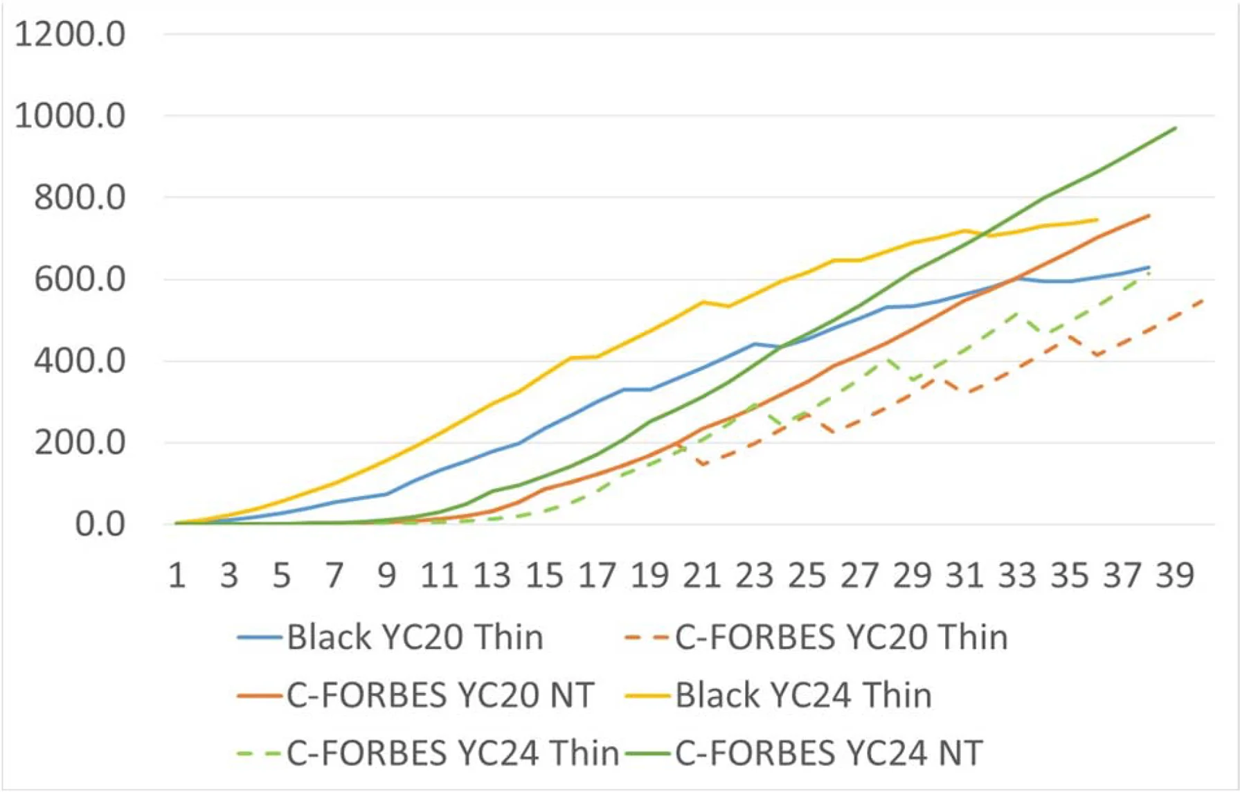
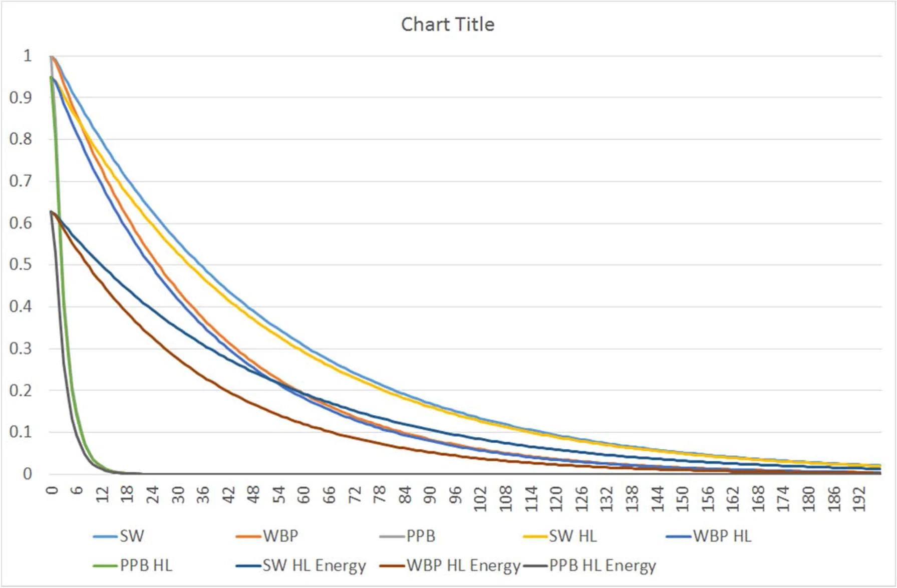
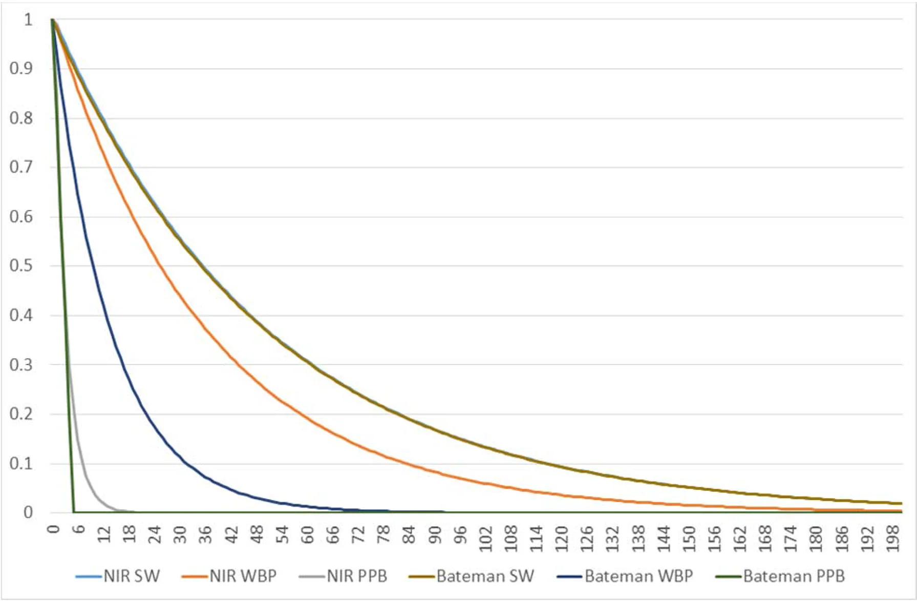
References

(1977). Operational Directive (1/77) “Rotation Lengths and Thinning Regimes for Conifers” Forest and Wildlife Service.
Asada, R, Cardellini, G, Mair-Bauernfeind, C, Wenger, J, Haas, V, Holzer, D, Stern, T (2020). Effective bioeconomy? A mrio-based socioeconomic and environmental impact assessment of generic sectoral innovations. Technological Forecasting and Social Change, 153 . https://doi.org/10.1016/j.techfore.2020.119946
Bach, S, Kohlhaas, M, Meyer, B, Praetorius, B, Welsch, H (2002). The effects of environmental fiscal reform in Germany: A simulation study. Energy Policy, 30 , 803–811. https://doi.org/10.1016/S0301-4215(02)00005-8
Baker, K, Bull, G, Baylis, K, Barichello, R (2017). Towards a Theoretical Construct for Modelling Smallholders’ Forestland-Use Decisions: What Can We Learn from Agriculture and Forest Economics?. Forests, 8 , 345–366. https://doi.org/10.3390/f8090345
Bateman, IJ (1996). An Economic Comparison of Forest Recreation, Timber and Carbon Fixing Values with Agriculture in Wales: A Geographical Information Systems Approach. PhD Thesis, Department of Economics, University of Nottingham.
Bateman, IJ, Lovett, AA (2000). Estimating and valuing the carbon sequestered in softwood and hardwood trees, timber products and forest soils in Wales. Journal of Environmental Management, 60 , 301–323. https://doi.org/10.1006/jema.2000.0388
Berry, A (2019). The distributional effects of a carbon tax and its impact on fuel poverty: A microsimulation study in the french context. Energy Policy, 124 , 81–94. https://doi.org/10.1016/j.enpol.2018.09.021
Binner, A, Day, B, Owen, N, Bateman, I, Smith, G, Collings, G, Haddrell, L, Luizo, L, Fezzi, C (2019). Chapter 3b in Natural Environment Valuation Online Tool (NEVO). Land, Environment, Economics and Policy (LEEP) Institute.
Black, K (2016). Description, calibration and validation of the CARBWARE single-tree-based stand simulator. Forestry, 89 , 55–68. https://doi.org/10.1093/forestry/cpv033
Black, K, Byrne, KA, Mencuccini, M, Tobin, B, Nieuwenhuis, M, Reidy, B, Bolger, T, Saiz, G, Green, C, Farrell, ET, Osborne, B (2009). Carbon stock and stock changes across a Sitka spruce chronosequence on surface-water gley soils. Forestry, 82 , 255–272. https://doi.org/10.1093/forestry/cpp005
Black, K, Hendrick, E, Gallagher., G, Farrington, P (2012). Establishment of Irelands projected reference level for forest management for the period 2013-2020 under article 3.4 of the Kyoto Protocol. Irish Forestry, 69 , 7–33.
Black, K, Tobin, B, Saiz, G, Byrne, K, Osbourne, B (2004). Improved estimates of biomass expansion factors for Sitka spruce. Irish Forestry, 50–65.
Boulanger, P, Dudu, H, Ferrari, E, Mainar, AJ, Ramos, MP (2020). Effectiveness of Fertilizer Policy Reforms to Enhance Food Security in Kenya: A Macro-Microsimulation Analysis. Applied Economics, 1–21. https://doi.org/10.1080/00036846.2020.1808180
Byrne, KA, Farrell, EP (2005). The effect of afforestation on soil carbon dioxide emissions in blanket peatland in Ireland. Forestry, 78 , 217–227. https://doi.org/10.1093/forestry/cpi020
Cannell, M, Cape, J (1991). In Forestry Expansion.
Carauta, M, Latynskiy, E, Mössinger, J, Gil, J, Libera, A, Hampf, A, Monteiro, L, Siebold, M, Berger, T (2017). Can preferential credit programs speed up the adoption of low-carbon agricultural systems in Mato Grosso, Brazil? Results from bioeconomic microsimulation. Regional Environmental Change, 18 , 117–128. https://doi.org/10.1007/s10113-017-1104-x
Clinch, JP (1999). Economics of Irish Forestry: Evaluating the Returns to Economy and Society. COFORD. Dublin.
Corbyn, IN, Crockford, KJ, Savill, PS (1988). The estimation of the branchwood component of broadleaved woodlands. Forestry, 61 , 193–204. https://doi.org/10.1093/forestry/61.3.193
Cornwell, A, Creedy, J (1996). Carbon taxation, prices and inequality in Australia. Fiscal Studies, 17 , 21–38. https://doi.org/10.1111/j.1475-5890.1996.tb00492.x
(2015). Afforestation Grant and Premium Schemes. Forest Service of the Department of Agriculture, Food and Marine.
(2018). Department of Agriculture Forest and the Marine.
Dewar, RC, Cannell, MG (1992). Carbon sequestration in the trees, products and soils of forest plantations: An analysis using UK examples. Tree Physiology, 11 , 49–71. https://doi.org/10.1093/treephys/11.1.49
Doole, GJ, Marsh, D, Ramilan, T (2013). Evaluation of agri-environmental policies for reducing nitrate pollution from New Zealand dairy farms accounting for firm heterogeneity. Land Use Policy, 30 , 57–66. https://doi.org/10.1016/j.landusepol.2012.02.007
(2019). Public Spending Code Supplementary Guidance - Measuring & Valuing Changes in Greenhouse Gas Emissions in Economic Appraisals. Department of Public Expenditure and Reform, December 2019. https://www.gov.ie/en/publication/public-spending-code/.
Duesberg, S, Dhubháin, ÁN, O’Connor, D (2014). Assessing policy tools for encouraging farm afforestation in Ireland. Land Use Policy, 38 , 194–203. https://doi.org/10.1016/j.landusepol.2013.11.001
Duesberg, S, O’Connor, D, Dhubháin, ÁN (2013). to plant or not to plant—irish farmers’ goals and values with regard to afforestation. Land Use Policy, 32 , 155–164. https://doi.org/10.1016/j.landusepol.2012.10.021
Dunford, RW, Smith, AC, Harrison, PA, Hanganu, D (2015). Ecosystem service provision in a changing Europe: Adapting to the impacts of combined climate and socio-economic change. Landscape Ecology, 30 , 443–461. https://doi.org/10.1007/s10980-014-0148-2
Edwards, PN, Christie, JM (1981). Yield Models for Forest Management, Forest Commission Booklet 48. London: HMSO.
Farrelly, NJ (2011). Doctoral dissertation, University College Dublin.
Hennessy, T, Moran, B, Kinsella, A, Quinlan, G (2013). Teagasc Agricultural Economics and Farm Surveys Department, Athenry, Co.
Herbohn, J, Emtage, N, Harrison, S, Thompson, D (2013). The Australian Farm Forestry Financial model. Australian Forestry, 72 , 184–194. https://doi.org/10.1080/00049158.2009.10676300
Hynes, S, Morrissey, K, O’Donoghue, C, Clarke, G (2009). A spatial micro-simulation analysis of methane emissions from Irish agriculture. Ecological Complexity, 6 , 135–146. https://doi.org/10.1016/j.ecocom.2008.10.014
Hynes, S, O’Donoghue, C (2014). Handbook of Microsimulation Modelling.
Im, EH, Adams, DM, Latta, GS (2007). Potential impacts of carbon taxes on carbon flux in western Oregon private forests. Forest Policy and Economics, 9 , 1006–1017. https://doi.org/10.1016/j.forpol.2006.09.006
(2006). Intergovernmental Panel on Climate Change Guidelines for National Greenhouse Gas Inventories. Cambridge, UK: IPCC.
(2013). Interagency working group on social cost of carbon, US government, technical support document: Technical update of the social cost of carbon for regulatory impact analysis under executive order 12866, May 2013. https://www.federalregister.gov/documents/2013/11/26/2013-28242/technical-support-document-technical-update-of-the-social-cost-of-carbon-for-regulatory-impact.
Jacobsen, H, Birr-Pedersen, K, Wier, M (2003). Distributional implications of environmental taxation in Denmark. Fiscal Studies, 24 , 477–499.
Jönsson, M, Snäll, T, Leverkus, AB (2020). Ecosystem service multifunctionality of low‐productivity forests and implications for conservation and management. Journal of Applied Ecology, 57 , 695–706. https://doi.org/10.1111/1365-2664.13569
Kilbride, CM, Byrne, KA, Gardiner, lJ (1999). In: Carbon Sequestration and Irish/Orests. Dublin: COFORD.
Knaggs, G, O’Driscoll, E (2017). Woodflow and forest-based biomass energy use on the island of Ireland (2016). http://www.coford.ie/media/coford/content/publications/2016/00795CCNWoodflowPP48Web070318.pdf.
van Kooten, GC, Laaksonen-Craig, S, Wang, Y (2009). A meta-regression analysis of forest carbon offset costs. Canadian Journal of Forest Research, 39 , 2153–2167. https://doi.org/10.1139/X09-139
Kurz, WA, Dymond, CC, White, TM, Stinson, G, Shaw, CH, Rampley, GJ, Smyth, C, Simpson, BN, Neilson, ET, Trofymow, JA, Metsaranta, J, Apps, MJ (2009). CBM-CFS3: A model of carbon-dynamics in forestry and land-use change implementing IPCC standards. Ecological Modelling, 220 , 480–504. https://doi.org/10.1016/j.ecolmodel.2008.10.018
Lanigan, G, Donnellan, T, Hanrahan, K, Paul, C, Shalloo, L, Krol, D, Forrestal, D, O’Brien, D, Ryan, M, Murphy, P, Caslin, B, Finnan, J, Boland, A, Upton, J, Richards, K (2019). An Analysis of Abatement Potential of Greenhouse Gas Emissions in Irish Agriculture 2021-2030.
McDonagh, J, Farrell, M, Ryan, M (2011). Missed opportunity or cautionary steps?. European Countryside, 236–251.
Monteith, JL (2002). Fundamental equations for growth in uniform stands of vegetation. Agricultural and Forest Meteorology, 104 , 5–11.
Moore, FC, Diaz, DB (2015). Temperature impacts on economic growth warrant stringent mitigation policy. Nature Climate Change, 5 . https://doi.org/10.1038/nclimate2481
Morison, J, Matthews, R, Miller, G, Perks, M, Randle, T, Vanguelova, E, White, M, Yamulki, S (2012). Understanding the carbon and greenhouse gas balances of forests in Britain. Forestry Commission Research Report. Forestry Commission, Edinburgh.
(2018). http://files.nesc.ie/nesc_secretariat_papers/No_15_CBA_Env_and_ClimateChange.pdf. http://files.nesc.ie/nesc_secretariat_papers/No_15_CBA_Env_and_ClimateChange.pdf.
(2012). Ireland’s National Inventory Report. Wexford, Ireland: Environmental Protection Agency.
(2015). Ireland’s National Inventory Report. Wexford, Ireland: Environmental Protection Agency.
(2018). Ireland’s National Inventory Report. Wexford, Ireland: Environmental Protection Agency.
(2019). Ireland’s National Inventory Report. Wexford, Ireland: Environmental Protection Agency.
Nordhaus, W (2014). Estimates of the social cost of carbon: Concepts and results from the DICE-2013R model and alternative approaches. Journal of the Association of Environmental and Resource Economists, 1 , 273–312. https://doi.org/10.1086/676035
(2016). Better Policies for Sustainable Development 2016: A New Framework for Policy Coherence. Paris: Organisation for Economic Co-operation & Development Publishing.
O’Donoghue, C (2017). Farm-Level Microsimulation Modelling. Cham: Palgrave Macmillan.
O’Donoghue, C, Chyzheuskaya, A, Grealis, E, Kilcline, K, Finnegan, W, Goggins, J, Hynes, S, Ryan, M (2019). Measuring ghg emissions across the agri-food sector value chain: The development of a bioeconomy input-output model. International Journal on Food System Dynamics, 55–85.
O’Malley, S, Roantree, B, Curtis, J (2020). Carbon Taxes, Poverty, and Compensation Options.
Pannell, DJ, Claassen, R (2020). The Roles of Adoption and Behavior Change in Agricultural Policy. Applied Economic Perspectives and Policy, 42, 31–41. https://doi.org/10.1002/aepp.13009
Phillips, H (1998). Report Commissioned by Coillte Forests.
Phimmavong, S, Keenan, RJ (2020). Forest plantation development, poverty, and inequality in Laos: A dynamic CGE microsimulation analysis. Forest Policy and Economics, 111 . https://doi.org/10.1016/j.forpol.2019.102055
Pingoud, K, Wagner, F (2006). Methane emissions from landfills and carbon dynamics of harvested wood products: The first-order decay revisited. Mitigation and Adaptation Strategies for Global Change, 11 , 961–978. https://doi.org/10.1007/s11027-006-9029-6
Rahman, A (2018). New Directions in Microsimulation.
Ramilan, T, Scrimgeour, F, Marsh, D (2011). Analysis of environmental and economic efficiency using a farm population micro-simulation model. Mathematics and Computers in Simulation, 81 , 1344–1352. https://doi.org/10.1016/j.matcom.2010.04.018
Richardson, J, Hennessy, T, O’Donoghue, C (2014). Handbook of MicroSimulation.
Romero, G, Álvarez-Espinosa, A, Calderón, S, Ordóñez, A (2018). Redistributive impacts of a carbon tax in Colombia: The link between models of microsimulations and general equilibrium. Lecturas de Economía, 89 , 163–198.
Rosas-Flores, JA, Bakhat, M, Rosas-Flores, D, Fernández Zayas, JL (2017). Distributional effects of subsidy removal and implementation of carbon taxes in mexican households. Energy Economics, 61 , 21–28. https://doi.org/10.1016/j.eneco.2016.10.021
Ryan, M, McCormack, M, O’Donoghue, C, Upton, V (2014). The role of subsidy payments in the uptake of forestry by the typical cattle farmer in Ireland from 1984 to 2012. Irish Forestry, 92–112.
Ryan, M, O’Donoghue, C (2019). Developing a microsimulation model for farm forestry planting decisions. International Journal of Microsimulation, 12 .
Ryan, M, O’Donoghue, C, Hynes, S (2018). Heterogeneous economic and behavioural drivers of the farm afforestation decision. Journal of Forest Economics, 33 , 63–74. https://doi.org/10.1016/j.jfe.2018.11.002
Ryan, M, O’Donoghue, C, Phillips, H (2016). Modelling financially optimal afforestation and forest management scenarios using a bio-economic model. Open Journal of Forestry, 06 , 19–38. https://doi.org/10.4236/ojf.2016.61003
Sedjo, RA (2001). . Resources for the Future Discussion Papers.
Serret, Y, Johnstone, N (2006). Distributional Effects of Environmental Policy: Conclusions and Policy Implications.
Smith, S, Braathen, NA (2015). Monetary carbon values in policy appraisal: An overview of current practice and key issues. OECD Environment Working Papers.
Soimakallio, S, Kalliokoski, T, Lehtonen, A, Salminen, O (2021). On the trade-offs and synergies between forest carbon sequestration and substitution. Mitigation and Adaptation Strategies for Global Change, 26 . https://doi.org/10.1007/s11027-021-09942-9
Stern, N (2007). Stern Review: The Economics of Climate Change. London, UK: HM treasury.
Symons, E, Proops, J, Gay, P (1994). Carbon taxes, consumer demand and carbon dioxide emissions: A simulation analysis for the UK. Fiscal Studies, 15 , 19–43. https://doi.org/10.1111/j.1475-5890.1994.tb00195.x
(2019). Coillte Annual Contracted Standing Sales (€/M3) by Average Tree Size and per Year.
(2021). Teagasc Forest Carbon Tool.
Temperli, C, Blattert, C, Stadelmann, G, Brändli, UB, Thürig, E (2020). Trade-offs between ecosystem service provision and the predisposition to disturbances: A nfi-based scenario analysis. Forest Ecosystems, 7 , 1–17. https://doi.org/10.1186/s40663-020-00236-1
Thompson, DA, Matthews, RW (1989). The storage of carbon in trees and timber. Forestry Commission Research Information Note, 160 .
Thorne, FS, Fingleton, W (2006). Examining the relative competitiveness of milk production: An irish case study (1996–2004. Journal of International Farm Management, 3 , 49–61.
Tobin, B, Nieuwenhuis, M (2007). Biomass expansion factors for Sitka spruce (Picea sitchensis (Bong.) Carr.) in Ireland. European Journal of Forest Research, 126 , 189–196. https://doi.org/10.1007/s10342-005-0105-3
(2019). World Population Prospects 2019: Highlights, United Nations, Department of Economic and Social Affairs, Population Division.
Wellock, ML, LaPerle, CM, Kiely, G (2011). What is the impact of afforestation on the carbon stocks of irish mineral soils?. Forest Ecology and Management, 262 , 1589–1596. https://doi.org/10.1016/j.foreco.2011.07.007
Yemshanov, D, McCarney, G. R, Hauer, G, Luckert, M. M, Unterschultz, J, McKenney, D. W (2015). A real options-net present value approach to assessing land use change: A case study of afforestation in Canada. Forest Policy and Economics, 50 , 327–336.
(2006). The Distributional Effects of Environmental Policy. OECD Publishing.

Article and author information

Author details

Mary Ryan
Teagasc, Athenry, Co. Galway, Ireland
For correspondence: Mary.ryan@teagasc.ie
ORCID iD: 0000-0001-8395-6953
Cathal O’Donoghue
National University of Ireland, Galway, Ireland
ORCID iD: 0000-0003-3713-5366

Funding

The authors are grateful for funding from the Sustainable Energy Authority of Ireland under the BIO-CIRCLE Project (SEAI RDD235).

Acknowledgements

This research was supported by the SeQUEsTER Project (Scenarios Quantifying land Use & Emissions Transitions towards Equilibrium with Removals) (EPA Research Programme 2014-2020). The EPA Research Programme is a Government of Ireland initiative funded by the Department of Communications, Climate Action and Environment.

Although every effort has been made to ensure the accuracy of the material contained in this journal article, complete accuracy cannot be guaranteed. Neither the Environmental Protection Agency nor the authors accept any responsibility whatsoever for loss or damage occasioned or claimed to have been occasioned, in part or in full, as a consequence of any person acting or refraining from acting, as a result of a matter contained in this journal article.

Publication history

Version of Record published: April 30, 2021 (version 1)

Copyright

This article is distributed under the terms of the Creative Commons Attribution License, which permits unrestricted use and redistribution provided that the original author and source are credited.

1. Introduction

2. Theoretical Framework

2.1. Private (financial) impact of farm afforestation

2.2. The Public Good (carbon) Impact of Farm Afforestation

3. Methodology

3.1. C-ForBES Microsimulation Framework6

3.2. C-ForBES Agricultural GHG emissions estimation

3.3. C-ForBES Forest Carbon Estimation

4. Data and Summary Statistics

4.1. Carbon Models, Assumptions and Validation

5. Results and Discussion

5.1. Carbon Sequestration

5.2. Private and Social Returns to Land use Change from Agriculture to Forestry

5.3. Sensitivity Analyses

5.4. Distribution of Private and Social Returns

5.5. Impact of substitution of trees for livestock - area of livestock emissions offset by a hectare of different types of afforestation

6. Conclusions

Footnotes

1.

2.

3.

4.

5.

6.

7.

8.

9.

10.

11.

12.

13.

14.

15.

16.

Appendix A: Agricultural parameters

Appendix B: Forest Parameters

Appendix C: An Examination of Variability in Methodological Assumptions

References

Article and author information

Author details

Mary Ryan

Cathal O’Donoghue

Funding

Acknowledgements

Publication history

Copyright

3.1. C-ForBES Microsimulation Framework⁶