
Jump to
1. Introduction
In discussions of future policies, policy-makers would like to obtain information about the effects of the policies in question compared to a “no change” benchmark. For example, they would like to know the costs and distributional effects of prospective changes in taxes and benefits. Microsimulation modelling tools are commonly used to provide such information. The capacity of these models to forecast the effects of policies that do not currently exist, but might do so in the future, also referred to as “what if” analysis, is widely acknowledged (Bourguignon and Ferreira, 2003; Bourguignon and Spadaro, 2006; Figari et al., 2015).
Hence, microsimulation models are integral parts of the policy-making process worldwide. For example, in the U.S., the Congressional Budget Office, the Joint Committee on Taxation and the Office of Tax Analysis develop and operate several microsimulation models (Joint Committee on Taxation, 2011). In Europe, a tax-benefit model for the countries of the European Union has been developed – EUROMOD (Sutherland and Figari, 2013). A selection of other models include NBER’s TAXSIM (Feenberg and Coutts, 1993) and the Urban-Brookings Tax Policy Center Microsimulation Model (Rohaly et al., 2005) for the U.S., IFS’s TAXBEN (Waters, 2017) for the U.K., MITTS of the University of Melbourne (Creedy et al., 2001) for Australia, Statistics Sweden’s FASIT (Helgeson et al., 2018), and the Danish Ministry of Finance’s Law Model (Finansministeriet, 2003).
In Norway, the microsimulation model system LOTTE has been used for several decades to assist in tax policy-making. The system is part of the portfolio of prediction models developed and maintained by the Research Department of Statistics Norway. Other models include the Keynesian macro model KVARTS (Boug et al., 2023), the DSGE model NORA (Aursland et al., 2020), the dynamic microsimulation model MOSART (Andreassen et al., 2020), the general equilibrium model SNOW (Fæhn et al., 2020), and the general equilibrium model for analysis of fiscal sustainability problems, DEMEC (Holmøy and Strøm, 2017). The models have in common that they are developed and maintained by staff at Statistics Norway. However, the operation of models in the policy-making process varies somewhat: some models are exported to, and operated by, personnel at the Ministry of Finance, while others are kept at and operated by Statistics Norway.
In this paper we describe the models of the LOTTE system – the static microsimulation models of Statistics Norway, designed to simulate the effects of changes in the taxation of individuals and households; see Aasness et al. (2007) for a previous model documentation. We characterize the models of the LOTTE system as static because they have no dynamic elements.1 However, non-dynamic does not mean non-behavioral, and as we will describe, the LOTTE system includes both behavioral and non-behavioral models.
Currently, there are three defined models belonging to the LOTTE system, and we present each of them in turn.2 In addition to describing the design of each model,3 we explain how they are used to assist in policy-making and how they have been used in discussions of broader tax policy questions for an international audience, i.e., in international academic journals.
First, the workhorse of the LOTTE model system is the standard non-behavioral (or arithmetic) tax-benefit model LOTTE-Skatt.4 It has been in extensive use for more than five decades, since its introduction in the early 1970s. Designated Statistics Norway personnel operate the model on a daily basis to assist in the policy-making process. Although a main focus here is on its practical use in the policy-making, the model has proven useful in academic work too. For example, the model has been used in discussions of tax redistributional effects in Lambert and Thoresen (2009), which we will return to later in this paper.
Second, the behavioral counterpart to LOTTE-Skatt is LOTTE-Arbeid, as this model predicts labor supply effects of changes in the personal income tax.5 Behavioral microsimulation models are often based on estimation of structural equations, which means that demanding econometric work is typically involved. The discrete choice labor supply model of van Soest (1995) represents a dominant empirical approach in practical work, see for example Blundell and Hoynes (2004), Kalb (2010), and de Boer and Jongen (2023). LOTTE-Arbeid builds on a particular discrete choice labor supply model based on the concept of “job choice”, developed over several decades by econometricians of Statistics Norway and the University of Oslo; see Dagsvik (1994), Aaberge et al. (1995), Dagsvik et al. (2014), and Dagsvik and Jia (2016).
Third, the model LOTTE-Konsum was developed to describe distributional effects of changes in the commodity taxation (Aasness et al., 2002).6 The empirical strategy behind LOTTE-Konsum is based on an imputation method, where household expenditures are derived from a system of Engel functions, and assigned to households on the basis of demographic information. In LOTTE-Konsum the budget shares for each household are calculated for the baseline (benchmark) situation and used to calculate a household-specific price index. The simulations of the distributional effects of changes in the commodity taxation are then carried out by letting the price index reflect the tax changes. Revenue effects of the same changes are obtained from separate revenue models, run by the Ministry of Finance.
The LOTTE model portfolio shares important similarities with many of the other models, referred to above. For example, EUROMOD now includes a labor market adjustment add-on (EUROLAB), in addition to the tax-benefit calculator (Christl et al., 2023) and MITTS (of the University of Melbourne) includes both a tax-benefit model and a behavioral labor supply module. Thus, the case where a labor supply module works in conjunction with a non-behavioral tax-benefit calculator, such as the LOTTE-Skatt and LOTTE-Arbeid combination, is rather common. Perhaps the most idiosyncratic member of our model collection is LOTTE-Konsum. There are other models also calculating effects of changes in indirect taxes, such as TAXBEN of the UK, but the imputation method of LOTTE-Konsum is (to our knowledge) rather unique.
The paper is organized as follows. In Section 2 we give a brief historical overview of the development of the models in the LOTTE system. Section 3 then describes the tax-benefit module for personal income tax simulations, LOTTE-Skatt, Section 4 presents the labor supply module, LOTTE-Arbeid, and Section 5 presents the module that describes the distributional effects of commodity taxation, LOTTE-Konsum. Each model presentation includes descriptions of how the model is used in the decision-making process, as well as examples of how the models are used to reach out to a wider academic audience. Section 6 provides concluding remarks.
2. Model development
The development of a tax-benefit model for Norway started in the early 1970s – the first version was operational and documented in 1972 (Rosenqvist, 1972). The model was named LOTTE after its founder, CharLOTTE Rosenqvist. Later, when other modules were developed, it was renamed LOTTE-Skatt. In those early years, model simulations were executed by means of data tapes and punch cards using FORTRAN programming. Model samples in the early days were small, about 13,000 in 1967 (the individual as the unit). Despite this the running time was very high (about 45 minutes). Due to lack of detailed information about taxpayers’ income and wealth, as well as a small sample size, the first version of the model was probably not very accurate.
The LOTTE model was revised in 1981, documented in Hovland and Røyne (1982). A new feature was that a terminal could be used instead of punch cards. Data improvements meant that more detailed information about different elements of total income and total wealth was used, enabling more comprehensive simulations of the personal tax system. The main unit was still the taxpayer, but information about household formation was added using data from three household sample surveys (1970, 1973, and 1976).
New advances in IT and increased demand for simulations by policy-makers led to further revisions of the model (Nygaard, 1988; Lian, 1991). It was decided to change the programming language from FORTRAN to SAS (Statistical Analysis System). In 1991 the model was redesigned to run on the UNIX operating system, and a tax simulation was executed within approximately 2.5 minutes. The input data that covered only around 0.5 percent of the population were expanded to include information on different types of transfers and pensions, which led to the development of a pension/transfer module (Arneberg, 1994). This module was updated for only a few years and then terminated.7 Another short-lived module was called LOTTE-AS, developed to simulate effects of changes in corporate income taxation, after Norway adopted a version of the dual income tax in 1992 (Aarbu and Lian, 1996).
The mid-90s saw the advent of LOTTE-Konsum, which simulates the distributional effects of changes in commodity taxation (Aasness et al., 2002). In contrast to LOTTE-Skatt, this model was not used for revenue calculations – only to describe distributional effects.
The third model in the LOTTE system, the labor supply model LOTTE-Arbeid, was introduced in 2008. This module is based on a particular structural discrete choice model resulting from seminal econometric work by staff at Statistics Norway and the University of Oslo for several decades prior to the initiation of LOTTE-Arbeid (Dagsvik, 1994; Aaberge et al., 1995).
The development of microsimulation models has benefited vastly from the revolution following from the exploitation of administrative registers for data purposes. The Register of Income Tax Returns was in place in 1993, but because information on household formation was derived by separate sample surveys, the number of persons in LOTTE-Skatt was small compared to the total population of Norway. However, from 2005, a unique address register for all dwellings in Norway made it possible to establish households on the basis of residential addresses. From then on, Income and wealth statistics for households (Statistics Norway, 2021) for the complete Norwegian population constitute the main data source for LOTTE-Skatt. We provide further information on the various data sources in Section 3.2.
Another important data innovation was a new valuation scheme for housing, in place from 2010. Before 2010, housing values were obtained from a register of historical tariff values, which implied that older dwellings got unrealistically low values. This resulted in legitimacy problems for the tax schemes based on these values, for example in the taxation of annual net wealth.8 Since 2010 the Norwegian Tax Administration has employed data sets for housing transactions and hedonic regression techniques to calculate values for each primary dwelling for tax purposes. The parameter estimates of the hedonic regression render predicted housing values based on characteristics such as geographical location, housing types, and size. Housing values are upgraded annually by means of data on new transactions.
The main reason for models being developed and operated by Statistics Norway is data restriction regulations, which bar people outside the research community from access to microdata.9 However, it was considered convenient to let the Ministry of Finance having access to their own version of LOTTE-Skatt, and in 2011 a simplified version of LOTTE-Skatt, named LOTTE-Aksess, was introduced. This model version prevents the model user from direct access to micro data.10 This means that although LOTTE-Skatt is located on a server at Statistics Norway and maintained by staff at Statistics Norway, a version of it can be operated by tax analysts at the Ministry of Finance. In 2021 a more user-friendly version of LOTTE-Aksess was made available for the Ministry of Finance, with a SharePoint site for ordering and with simulation results reported in Excel.
3. LOTTE-Skatt
3.1 Model design
The Norwegian non-behavioral tax-benefit model LOTTE-Skatt holds a key position in the decision-making system in Norway. The model is extensively used by the Ministry of Finance in preparing the budget, while the other political parties in the Storting (the Norwegian parliament) make particular use of the model to develop their alternative budget proposals after the proposed government budget has been presented. Simulation results are reported back to the opposition parties fairly promptly. Many of these simulations are done by staff at the Ministry of Finance through LOTTE-Aksess. More complicated tax changes and tax simulations for alternative budget proposals are executed by dedicated model operators at Statistics Norway.
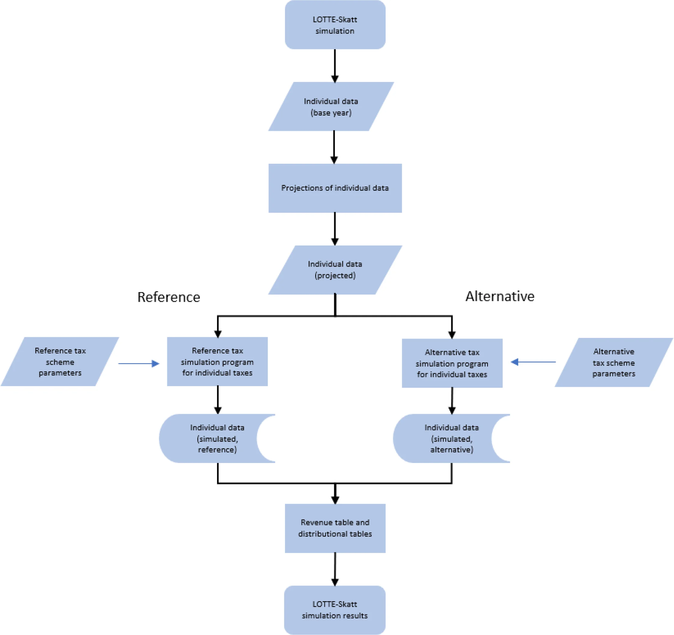
Figure 1 provides a graphical illustration of the different components of a standard LOTTE-Skatt tax simulation. A simulation consists of several elements and steps: individual input data (described in Section 3.2), a program that projects data for the year of interest (described in Section 3.3), a set of tax scheme parameters reflecting the tax legislation and a simulation program that applies the tax legislation to the individual data records.11 The results of a tax policy change simulation are compared to results of a reference simulation. For instance, when the policy-makers are preparing the next year’s budget, they compare effects of various tax-law changes to effects of a simulation based on this year’s tax-law, projected to the next budget year.
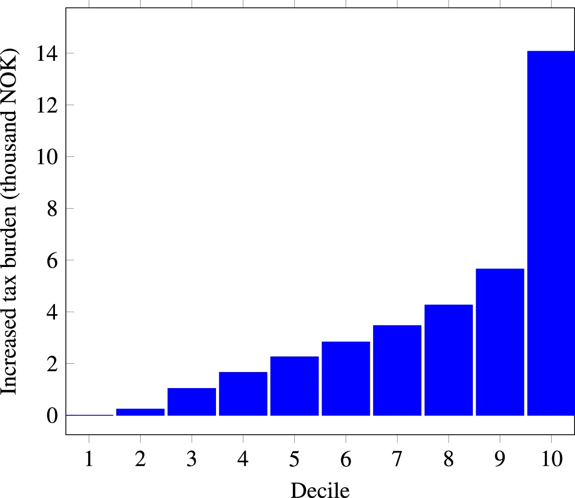
Standard model output of LOTTE-Skatt includes aggregate tax revenue effects and various descriptions of distributional effects. To illustrate this, we show simulation results for an increase in the net tax rate of the dual income tax scheme: the tax on ordinary income is increased by 1 percentage point, from 22 percent to 23 percent. Table 1 demonstrates how a standard revenue table would look like in this case, whereas Figure 2 provides a graphical depiction of an output table for distributional effects. The income distribution of Figure 2 (horizontal axis) is established by ranking individuals above the age of 16 by individual pre-tax income.12
| Alternative | Reference | Difference | |
|---|---|---|---|
| Income tax, municipal level | 237,079 | 220,840 | 16,238 |
| Income tax, state level | 136,401 | 136,401 | 0 |
| Social insurance tax | 178,102 | 178,102 | 0 |
| Bracket tax | 100,732 | 100,732 | 0 |
| Wealth tax, municipal level | 20,248 | 20,248 | 0 |
| Wealth tax, state level | 9,731 | 9,731 | 0 |
| - Tax red., housing savings scheme for young taxpayers | 580 | 580 | 0 |
| - Tax red., pensioners | 13,171 | 13,110 | 61 |
| - Tax red. in the north (North-Troms and Finnmark) | 1,133 | 1,119 | 14 |
| Total taxes | 667,409 | 651,246 | 16,163 |
| - Cash-for-care | 1,377 | 1,377 | 0 |
| - Child benefit | 22,171 | 22,171 | 0 |
| - Additional child benefit (small children, single parents) | 44 | 44 | 0 |
| Total | 643,817 | 627,654 | 16,163 |
Notes: Standard output revenue table from a LOTTE-Skatt simulation. Simulation alternative compared to a 2023 reference using 2020 data (10% sample) projected to 2023.
3.2 Data
The primary data source of the model is the Income and wealth statistics for households (Statistics Norway, 2021), which is based on several administrative registers, including detailed income tax return data from the Norwegian Tax Administration. Data from the Norwegian Labour and Welfare Administration (NAV) provide information about family, pension, disability, unemployment and other social security benefits, and data on education level and education support are provided by the Register of Education and the Norwegian State Educational Loan Fund. Limited company ownership of real estate is calculated for each person using data from the Register of Shareholders and from tax returns of limited companies.
The individual person is the primary unit of the model population, but output can be presented in terms of effects on households too. Households are formed based on a unique address register for all dwellings in Norway (see Section 2), connecting individuals by residential unit.
The full data sample include all 5.5 million individuals (of the country), corresponding to 2.2 million households. In order to reduce computational time, we usually use a sample consisting of about 10 percent of all households. However, high-income households (gross income exceeding NOK 10 million) and the wealthiest households (net wealth of more than NOK 100 million) are always included in the sample, to avoid biases in the revenue calculations.13 Accordingly, these households get a weight of 1, whereas other households have a 10 percent chance of being selected and therefore get a weight of 10.14
Households are categorized into five socioeconomic groups depending on the status of the “head of the household”, defined as the person with highest income: i) wage earners (52% of our sample in 2021), ii) self-employed (2%), iii) pensioners (20%), iv) social security recipients (11%), and v) others (14%).
3.3 Projections of tax base and tax scheme
Data must be projected from the year of the data (base year) to the simulation year, typically a three year time span. For example, in the spring of 2023, we prepared a data set for the year 2021 to be employed in simulations with respect to the 2024-budget, made public in early October 2023. The projections (or nowcasting) consists of two steps. First, projections are made for economic variables such as income, income deductions and wealth for each person. Income variables and income deduction variables are categorized with respect to adjustment factors, as different factors are employed for different income variables, such as for wage income, pension income, social security benefits, self-employed income (business income) and capital income (interest income, dividends, and gains).
Second, sample weights are adjusted to account for changes in the number of households assigned to each of the five socioeconomic statuses (see Section 3.2). Other demographic changes from base year to simulation year are not taken into account, which means that, e.g., distributions of age, gender, and geographical location as well as marital, socioeconomic, occupational and employment statuses are assumed to be the same in the simulation year as in the base year. The factors used in the projections are based on different sources of information: data from Statistics Norway, such as the National Accounts, published information from the Norwegian Labour and Welfare Administration, and forecasts from the Ministry of Finance.
Similarly, variables representing the tax legislation for the current year (e.g., maximum and threshold values) are projected to the budget year. The method for uprating the tax scheme includes using estimates of wage growth and consumer price growth. Importantly, there is an established convention guiding the procedure to project the tax system from one year to the next (for example, in the spring of 2023 we established a 2024 tax scheme benchmark based on the 2023 tax law): the tax scheme is uprated to the next year under the condition that the ratio of the tax to the tax base, for a taxpayer with only standard income deductions, is close for the two years.
3.4 Model validation
In general, model simulation results may deviate from the actual taxation, as reflected in the income tax return. Discrepancies emerge because 1) the tax simulations are simplified and because 2) not all parts of the scheme are simulated. As a result model output results typically deviate from what we get from the administrative tax registers, for example in terms of the individual tax burden. Various tests of model performance are regularly executed to get a picture of the magnitude of deviations and to keep track of over time developments.
Table 2 shows a comparison of output from LOTTE-Skatt and output collected from the tax register for 2021. Thus, this illustrates the extent of inaccuracies due to simplified tax simulation procedures. The table shows that total taxes, as simulated by LOTTE-Skatt, is 0.2 percent higher (1.2 billion NOK) than the taxation reported in the registers. Deviations vary from -0.11% to 3.84%, depending on the type of tax. Moreover, deviations caused by not being able to include all components of the tax system in the simulations give additional discrepancies of a similar magnitude, implying that the total deviation is about 0.4 percent.
| LOTTE-Skatt | Tax reg. | Diff. in % | |
|---|---|---|---|
| Income tax, municipal level | 254,589 | 254,199 | 0.15 |
| Income tax, state level | 122,580 | 122,382 | 0.16 |
| Social insurance tax | 165,319 | 164,829 | 0.30 |
| Bracket tax | 81,829 | 81,772 | 0.07 |
| Wealth tax, municipal level | 14,989 | 14,911 | 0.52 |
| Wealth tax, state level | 3,212 | 3,199 | 0.40 |
| - Tax reduction, housing savings scheme for young taxpayers | 1,003 | 0,966 | 3.84 |
| - Tax reduction, pensioners | 14,213 | 14,229 | -0.11 |
| - Tax reduction in the north (North-Troms and Finnmark) | 1,069 | 1,068 | 0.10 |
| Total | 626,233 | 625,029 | 0.19 |
Notes: Both the simulated output from LOTTE-Skatt and the output from administrative tax registers are based on the population of all residents in 2021.
Furthermore, using the 10 percent sample (see Section 3.2) instead of the full population is also a source to discrepancy. The deviation in total taxes caused by employing the 10 percent sample in the simulations is generally small (less than 0.1 percent), but care has to be taken when studying highly disaggregated simulation output.
3.5 Use of LOTTE-Skatt in academic work
3.5.1 Fixed-income approach
In the following we present two studies that use LOTTE-Skatt in contributions aimed for the international academic literature. First, we refer to Lambert and Thoresen (2009), where the tax-benefit model is used to evaluate the contribution of the tax system to redistribution and tax progressivity over time. Next, in Section 3.5.2, we describe how measures of tax policy behavioral effects can be produced by feeding estimates of behavioral response into a non-behavioral tax-benefit model, illustrated by Jia et al. (2023).
Lambert and Thoresen (2009) evaluate the contribution of the tax system to redistribution and tax progressivity over time (1992–2004) by using a “fixed-income” approach: different tax-laws are applied to the same (fixed) pre-tax income distribution.15 They present results for several pre-tax income distribution bases – those of 1992, 1998 and 2004. For each of these data sets, individuals were subjected to taxation as per the tax legislation of 1992, 1995, 1998, 2001, and 2004. When tax rules are from a year different from the point of time of the pre-tax income distribution, all tax thresholds are adjusted by wage growth.
Figure 3 shows how the tax policies of the period 1992–2004 are evaluated by the fixed-income approach. Effects are measured in terms of the Blackorby–Donaldson index (BD index) of redistributional effect (Blackorby and Donaldson, 1984), decomposed into vertical and horizontal inequity effects (VR and HI). The BD index is founded on social welfare function reasoning, as it employs the index of Atkinson (1970), , as an inequality index, where is the (relative) inequality aversion parameter, capturing the concavity of the utility function of an assumed social decision-maker.16 Furthermore, the decomposition into vertical and horizontal effects is carried out in terms of two concepts of horizontal inequity – the so-called “classical” and the “no reranking” approaches (C and NR). The classical approach to horizontal inequity Atkinson (1970) measurement starts from a perception of the vertical effect as being the average effect of the tax system on the relative income differentials of pre-tax unequals (Musgrave, 1990; Aronson et al., 1994; Jenkins and Lambert, 1999). The “no reranking” procedure arises from the perception that if individuals are reranked by the tax schemes in the transformation from pre-tax income to post-tax income, this amounts to procedural unfairness (Plotnick, 1981; King, 1983; Jenkins, 1994).
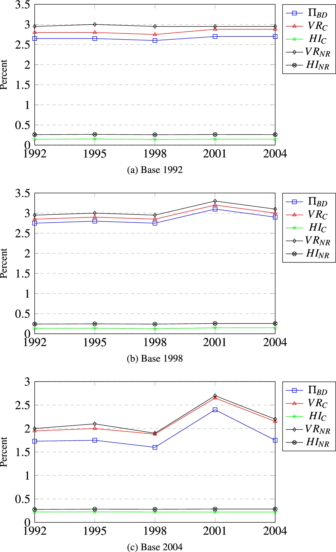
The most striking feature of Figure 3 is that the two lower panels pick up the temporary tax on dividends in 2001, whereas the upper panel does not. This follows from the small volume of dividend transfers in the 1992 data (less than NOK 2 billion), compared to pre-tax income distributions for 1998 and especially for 2004. These years have much higher taxable dividends, NOK 18 billion and NOK 63 billion, respectively. This is an example of the base dependence problem of the fixed-income approach. On balance, we find that the redistributional effect of the tax system is more or less unaltered from 1992 to 2004 – if anything, we see a small increase in the vertical redistribution over the period (for 1998 and 2004 base years).
3.5.2 Predicting behavioral effects of tax policy from external evidence
In Section 4 we return to how a fully developed structural behavioral model can accompany a tax-benefit model. Here, we describe an alternative approach where evidence from other empirical studies, for instance based on quasi-experimental evidence, can be used to describe the expected behavioral response of a prospective tax reform.17 We may refer to this latter procedure as making use of “external evidence” (Jia et al., 2023) or taking a reduced form approach (Ollonqvist et al., 2021).18 In practice, the method is founded on a simulation exercise where expected behavioral responses to a tax change are accounted for by adjusting the input of the non-behavioral tax-benefit model (as LOTTE-Skatt).
We illustrate the approach with an example in which a fifth bracket, for income of over NOK 2 million (EUR 200,000 and USD 230,000), and with a tax rate of 47.4 percent, is added to the Norwegian bracket tax scheme.19 The tax rate of the new bracket is 1 percentage point higher than the fourth bracket (46.4 percent). Given this example, only individuals with income over NOK 2 million are affected.
In the following, we describe the intensive margin responses:20 the marginal tax rate, , for each individual is simulated by increasing the individual’s earnings, , by a small amount ( = NOK 10),
where symbolizes tax. Then, if is the net-of-tax rate before the change, is the net-of-tax rate after the change, and is an earnings response estimate, we adjust pre-tax income by the factor
The reason for characterizing this approach as an “external evidence” procedure is that we obtain the response estimates from external sources. Based on evidence of the elasticity of taxable income (ETI) in the literature (Saez et al., 2012), we set . In selecting this estimate, we give more weight to estimates of the ETI based on Norwegian data, such as Aarbu and Thoresen (2001) and Thoresen and Vattø (2015).
Given the 1 percentage point change in the top marginal tax rate, the net-of-tax rate (at that level) increases by 1.9 percent. Furthermore, given the response estimate of 0.2, incomes over NOK 2 million (wage-income and self-employment income) are adjusted downward by 0.38 percent because of the tax increase.21 Then, estimates of post-reform taxes, disposable income, etc., before and after adjustment of pre-tax income, can be obtained from conventional LOTTE-Skatt simulations. The difference between simulation results with and without adjustments in pre-tax income defines the contribution from behavioral adjustments (to the tax change).
Table 3 presents the revenue effects of this tax change. The benchmark tax revenue is obtained by applying the tax rule of 2023 without the additional fifth bracket in the tax system. We find that the direct (non-behavioral) revenue effect of adding the fifth step is NOK 268 million. This revenue increase is counteracted by behavioral adjustments, reducing the revenue increase due to the tax change to NOK 156 million (268 minus 112), when behavioral adjustments at both the intensive and the extensive margins are taken into account. In total, this means that we get an estimate of the behavioral counteracting effect ratio of 0.42.22
| Total tax revenue | Diff. to benchmark | |
|---|---|---|
| Benchmark: 2023 tax rules without a 5th bracket | 578,134 | - |
| 2023 tax rules: | ||
| Direct (non-behavioral) effect | 578,402 | 268 |
| Intensive margin behavioral effect | -106 | |
| Extensive margin behavioral effect | -6 | |
| Direct and behavioral effects | 578,290 | 156 |
| Behavioral counteracting effect ratio | 0.42 |
Notes: Simulations generated by the Norwegian tax-benefit model LOTTE-Skatt, data for 2020 projected to 2023. Behavioral effects are taken into account with an ETI estimate of 0.2 at the intensive margin and 0.1 at the extensive margin. Source: Jia et al. (2023).
4. LOTTE-Arbeid
4.1 Labor supply responses
4.1.1 A discrete choice model based on the concept of “job choice”
Next, we turn to the labor supply module of the LOTTE system, LOTTE-Arbeid. The model simulates labor supply responses to alternative tax and transfer schemes based on a structural discrete choice labor supply model. In the category of structural labor supply modeling approaches, the discrete choice labor supply model, based on the random utility modeling framework (van Soest, 1995), has gained widespread popularity among public finance practitioners (Creedy and Kalb, 2005). This type of model can easily handle non-convex budget sets and two-earner households.
We use a specific discrete choice model based on the concept of “job choice” (Dagsvik, 1994; Aaberge et al., 1995; Dagsvik et al., 2014; Dagsvik and Jia, 2016). According to this framework, labor supply decisions are viewed as the outcomes of individuals choosing among jobs, with additional constraints on the set of available jobs.23 In this model, a labor supply decision is viewed as the choice of the most preferred job from a choice set of available jobs, where each job is characterized by non-pecuniary attributes, wage rate, and fixed job-specific hours of work. The jobs, choice sets and non-pecuniary job attributes (job-specific tasks to be performed, workplace locations and quality of work environment) are not observed by the researcher. Only the wage rate and the hours of work of the chosen jobs are observed.
Moreover, it is assumed that there may be more full-time jobs available than jobs with other working hours. The distribution of preferences for non-pecuniary job attributes is assumed to be independent of working hours. Hence, due to unobserved heterogeneity in preferences across individuals and latent jobs, it follows that more individuals will choose to work full-time than to work according to other schedules. The utilities of the jobs with any given workload are assumed to be randomly, independently and identically distributed (i.i.d.) across the set of available jobs.
The utility of disposable income, , hours of work, , and job indexed by is assumed to be
where means not working (in which case ), is a deterministic function and is a stochastic term that represents preferences for the non-pecuniary job attributes. For a given job, , the economic budget constraint is given by
where is hours of work in job , is the wage rate (individual-specific), is non-labor income and is the net-of-tax function. In addition to the economic budget constraint, an individual faces a specific choice set of available jobs, as mentioned above.
The cumulative distribution function of is assumed to be a Gumbel distribution.24 It then follows that the probability of choosing a job with hours of work , is equal to
where is the fraction of jobs with hours of work that is available to the individual, is an index that measures the size of the set of jobs that are available to the individual, and is the total set of available hours, which is assumed to be finite.
4.1.2 Data and estimation of the model
We assume that the deterministic part of the utility function can be represented by a Box-Cox function,
where represents the minimum or subsistence household-adjusted level of disposable income and is the maximum hours of work (total hours available minus sleep and rest). To account for observed heterogeneity in preferences, is allowed to depend on the individuals’ age and numbers of children in different age groups, whereas observed heterogeneity in job opportunities, is specified as a function of the individual’s education level. The function is assumed to be gender-specific and constant apart from possible peaks at part-time and full-time hours of work, as mentioned above. The model is estimated by the method of maximum likelihood, using samples of cross-sectional data from the Labor force survey. The data contains information on household incomes, wage rates, taxes, hours of work, schooling, as well as number and ages of children. The model is specified and estimated for prime-aged (25–62 years old) wage earners, separately for couples, single females and single males; see Dagsvik and Jia (2016), Rees et al. (2023), and Thoresen and Vattø (2015) for more details on estimation and estimation results.25
4.2 The labor supply model microsimulation module – LOTTE-Arbeid
The “job choice” model is the core of LOTTE-Arbeid. LOTTE-Arbeid work in conjunction with LOTTE-Skatt, in the sense that we transfer estimated parameters of the job choice model to the much larger LOTTE-Skatt data sample. In so doing we make the assumption that individuals of the LOTTE-Skatt data sample behave in the same way as those of the smaller sample used in the econometric estimations of labor supply (the Labour force survey), as long as they have the same observed characteristics. As the labor supply model is designed to provide simulation results for prime-aged wage earners (25–62 years old), we set the labor supply effects of other groups at zero. It is important to note that the model does not include behavioral responses for groups other than prime-aged wage earners, which means that the responses of self-employed individuals are neglected.26
Given the probabilistic nature of the labor supply model (following from the random utility discrete choice framework), we obtain predicted probability distributions for the discrete set of working hour alternatives for individuals, both pre- and post-reform. In particular, we calculate, for any given individual, values of the deterministic part of the utility function for each working hour alternative, using Equation (6), the estimated parameters, and observed characteristics. The corresponding probabilities, , are obtained by using Equation (5). Based on a predicted probability distribution for a discrete set of working hour alternatives, we obtain estimates of predicted hours of work, taxes paid, pre-tax income and other variables of interest. Furthermore, differences between probability distributions, pre- and post-reform, define labor supply effects of the tax change.
This procedure implies that we ignore the individual-level information on the unobserved error terms, , as we are mainly interested in aggregate responses. An alternative method is to follow Creedy and Kalb (2005) and Thoresen et al. (2010) and assume that the unobserved error terms are the same before and after the tax change.27
Table 4 presents our estimated labor supply elasticities with respect to the gross wage rate for females and males in couples (both own elasticities and cross elasticities) and for male and female singles, at both the extensive and the intensive margins (for females). In particular, the model predicts that females in couples are more responsive to wage changes than the other groups.28 This is a general finding in the labor supply literature (Whalen and Reichling, 2017; Eckstein et al., 2019; Keane, 2022), and the elasticity estimates are in line with other comparable microsimulation studies; see e.g., Bargain et al. (2014), and de Boer and Jongen (2023).29 Estimation results (not reported here) also show standard income response regularities, with negative labor supply response to increased non-labor income, such as increased child benefit.30 Note also that LOTTE-Arbeid has been extended to allow for state dependence in model framework that describes the timing of labor supply responses, see Jia and Vattø (2021). Results suggest that state dependence bring down the short-term (first-year) response to one-third of the full effect, and the full effect is reached after about five years.
| Female | Male | Female | Male | |
|---|---|---|---|---|
| Own wage | Own wage | Cross wage | Cross wage | |
| Individuals in couple | ||||
| Participation (ext. margin) | 0.135 | - | -0.048 | - |
| Hours cond. on working (int. margin) | 0.197 | 0.095 | -0.043 | -0.009 |
| Total elasticity | 0.332 | 0.095 | -0.091 | -0.009 |
| Single individuals | ||||
| Participation (ext. margin) | 0.012 | - | ||
| Hours cond. on working (int. margin) | 0.057 | 0.009 | ||
| Total elasticity | 0.069 | 0.009 |
Notes: The elasticities reflect the simulated percentage change (average across individuals) in the probability of participation (extensive margin) and working hours conditional on working (intensive margin) when the hourly wage rate is increased by one percent for all wage earners. Note that due to high male participation rates, we do not estimate extensive margin responses for males.
As a LOTTE-Arbeid simulation is both more complicated and time-consuming than a conventional LOTTE-Skatt simulation, the use of LOTTE-Arbeid in the Norwegian tax decision-making process is more limited. However, it is used to predict labor supply, revenue, and distributional effects of major reforms. An important output from the model is the information reported in Table 5, providing a rule of thumb for the degree of self-financing for a selection of tax changes. The ratio of self-financing is the ratio between the counteracting effect on revenue of labor supply adjustments due to a tax decrease and the estimated initial non-behavioral (or mechanical) revenue effect.31 This table is produced each year and presented in government reports, such as in Finansdepartementet (2023).32
| Tax change | Self-financing ratio, pct |
|---|---|
| Reduced rate bracket tax, bracket 3 | 10 |
| Increased threshold bracket tax, bracket 3 | 9 |
| Reduced rate ordinary income | 6 |
| Reduced rate social insurance tax | 5 |
| Reduced rate bracket tax, bracket 2 | 4 |
| Increased threshold bracket tax, bracket 2 | 2 |
| Increased threshold for maximum deduction in minimum standard deduction | 1 |
| Reduced rate bracket tax, bracket 1 | 0 |
| Increased threshold bracket tax, bracket 1 | 0 |
| Increased personal allowance | 0 |
| Increased rate minimum standard deduction | -16 |
Notes: For a tax decrease, the self-financing ratio is the ratio between the effect on revenue due to labor supply adjustments and the initial static (or mechanical) revenue effect estimate (standard tax-benefit model calculation). Source: Finansdepartementet (2023).
4.3 Validation of the labor supply model against estimates of the ETI literature
A key question in labor supply microsimulation is the extent to which the labor supply model provides valid results. It is fair to say that implausible structural estimates of taxes on labor supply have contributed to concern about the ability of structural models to generate robust predictions about the effects of policy change (Heckman and Urzúa, 2010; Imbens, 2010). In this perspective, results from (so-called) natural experiments serve as useful information sources for validation of prediction models (Blundell, 2006; Keane, 2010). Here, we demonstrate how simulation results from models like LOTTE-Arbeid can be tested against estimates of the ETI literature. The following is based on Thoresen and Vattø (2015).33
Some of the best examples of the strength of the structural discrete choice tool for economic planning, such as McFadden’s predictions regarding the use of a new train system in the San Francisco area (BART) (McFadden et al., 1977) and the prediction model developed by Todd and Wolpin (2006) through the PROGRESA project, have acquired their status through careful out-of-sample validations. This highlights that model validation is important and in the following we show how a validation can be done by obtaining estimates of the net-of-tax rate elasticity from a labor supply model simulation on working hours.34
As already denoted, the random utility framework of the discrete choice model involves generating a probability distribution for different working time options. In contrast, response estimates of the ETI literature are derived by marginal optimization, where response estimates reflect (somewhat simplified) the average responses of the “treated”, compared to “the less or not treated”. In order to obtain comparable figures, we therefore let the results of labor supply model simulations enter into a regression similar to that seen in the ETI literature, using the Norwegian tax reform of 2006 as a “natural experiment”. First, we use LOTTE-Arbeid to simulate the pre-reform and post-reform working hours for four groups of wage earners, the same groups as in Table 4, see results in Table 6. Then these results are converted into measures of growth in (simulated) working hours. In the replication of the ETI econometric framework, the variable for the change in the net-of-tax rate is derived from predicted income levels (hourly wage rate multiplied by predicted hours), and instrumented using similar methods to those of the ETI literature, i.e., the change in the net-of-tax rate for constant (predicted) pre-reform labor income.
| Pre-reform working hours | Post-reform working hours | Difference, % | |
| Single females | 35.20 (0.321) | 35.27 (0.322) | 0.18 |
| Single males | 38.95 (0.039) | 38.97 (0.040) | 0.04 |
| Females in couple | 32.13 (0.068) | 32.25 (0.068) | 0.36 |
| Males in couple | 38.60 (0.013) | 38.64 (0.014) | 0.11 |
Notes: Standard errors are obtained by non-parametric bootstrapping, 30 repetitions. Source: Thoresen and Vattø (2015).
In Table 7, estimates from the labor supply simulations are compared with the results of a standard ETI evaluation of the reform. We see that the panel data ETI figures for working hours are close to those obtained from the model simulations. In fact, there are no significant differences between the overall average estimates (for working hours); see the last row of Table 7. Furthermore, estimates (for all four groups) are found to be in the range 0.02–0.06. A difference of 0.04, which is the maximum difference (between results of the two methods) observed for working hours in Table 7 (single males), must be described as modest, both compared to the variation in elasticity estimates in the literature (see for example the review in Blundell and MaCurdy (1999)), and from a policy prediction perspective. Thus, it is claimed that the model performs well according to this validation. Of course, this does not mean that the simulation model is approved – it only means that the model has not been rejected by the present test, according to our judgment. It should also be noted that the ETI might potentially capture a broader set of responses, such as the effect of effort (wages), which is exogenously (fixed) in the standard labor supply model.35
| Discrete choice labor supply simulations, working hours | Panel data information | ||
|---|---|---|---|
| Working hours | Earned income | ||
| Single females | 0.018 (0.0005) | 0.032 (0.0037) | 0.020 (0.0051) |
| Single males | 0.062 (0.0027) | 0.023 (0.0055) | 0.039 (0.0054) |
| Females in couple | 0.026 (0.0001) | 0.051 (0.0046) | 0.031 (0.0045) |
| Males in couple | 0.015 (0.0005) | 0.016 (0.0059) | 0.053 (0.0034) |
| Weighted average | 0.026 (0.0012) | 0.028 (0.0053) | 0.041 (0.0043) |
Notes: The weighted averages are calculated by accounting for the number of observations in each group. Standard errors are obtained by using the delta method. Source: Thoresen and Vattø (2015).
5. LOTTE-Konsum
5.1 Model design
The purpose of LOTTE-Konsum is to simulate the direct (non-behavioral) distributional effects of changes in commodity taxation. For the same household population as in LOTTE-Skatt, the model contains a procedure for imputing consumption expenditure. A household-specific price index is used to represent the distributional effects of a tax change.
There is no observed consumption data in LOTTE-Konsum – consumption is imputed from micro econometric estimates of Engel functions and macro consumption data. Micro econometric estimates are based on the Consumer expenditure survey (Holmøy and Lillegard, 2014), and macro consumption is constructed by combining data from the national accounts (Bougroug, 2021) with forecasts from the macro model KVARTS (Boug et al., 2023). The first step of this procedure is to establish estimates of total expenditure for each household in the LOTTE-Skatt population. As our point of departure we assume that household has the consumption function,
where is total consumption expenditure, is the minimum consumption level, is disposable household income, and is the (common) marginal propensity to consume. By summing across households, we can derive the same expression in macro terms
where , , and . Given that we set minimum consumption levels and specify how they depend on the composition of household, we can calibrate the parameter from the aggregate disposable income and aggregate expenditure in the economy. This enables us to impute the total consumption in each household. Note that the marginal propensity to consume (and save), is constant. However, as there are minimum consumption levels, low-income households save less of their income than high-income households.
The next step is to distribute the total consumption of each household into different consumer goods. We start with the following Engel function for each good, ,
where and are the consumption and minimum consumption, respectively, of good , whereas is the marginal budget share.36 We assume that the minimum consumption of goods depends linearly on the number of children () and adults (),
Hence, we have an Engel function with demographic variables. By summing across households we get
where , . Given that we have information on macro budget shares, the Engel elasticities and the effects of adults and children on demand, we can calibrate the constant, , and assign expenditure per household for each good.37
A well-known problem when imputing consumption for low-income households is that some goods end up with negative consumption (Decoster et al., 2011). For these households, we proceed by setting consumption equal to zero for goods with negative consumption. However, this means that we end up with too high total expenditure for the household. We use an iterative procedure to adjust for this until total household expenditure is back at the initial level. Although we end up with many corner solutions, this ensures that the aggregate household expenditure for different goods in the economy is exactly equal to the macro data estimates.
Furthermore, it should be noted that the imputation of consumption implies that households have homogeneous preferences, given their income and the number of children and adults in the household. For example, this means that alcohol consumption is determined only by income level and household composition, and thus do not vary by other differences in preferences.38
Estimates of the distributional effects of a tax policy change are obtained by assigning to each household a household-specific price index. In practice, this means that based on the imputed budget shares, the Laspeyres formula is used to compute a household-specific price index for each household. The household-specific price index provides a good approximation of a “true cost of living index” for small price changes from the baseline situation for each household. Thus, the effects of a change in a commodity tax (or a commodity price) on the standard of living of each household, and each individual belonging to the household, is defined as total expenditure (possibly adjusted for economies of scale) divided by the household’s price index. Finally, it is worth noting that this approach makes it possible to consider the distributional effects of changes in direct and indirect taxation simultaneously.
A key advantage of the model concept is that it combines several sources of data, both micro and macro. Consumer expenditure surveys are often associated with substantial uncertainty, as samples are often small and contaminated with non-response bias. Also, consumption of more sensitive goods, such as tobacco and alcohol, is probably under-reported (Browning et al., 2014; Crossley and Winter, 2015). Rather than using observed data directly from a consumer expenditure survey, LOTTE-Konsum is employed to establish underlying stable patterns or trends by means of microeconometric studies, as reflected by Engel elasticity estimates. Moreover, since we use macro data to calibrate, the model results match macro estimates of consumption expenditure. All this ensures stability over time, which is an important quality of a model used on an annual basis by policy-makers.
There are currently 30 consumer goods in the model, but this is easily changed, given the specific policy question and availability of econometric estimates.39 This makes the model flexible, which is a clear advantage for policy-makers with a shifting focus on different commodity taxes.
5.2 Output in the decision-making process
In Tables 8 and 9 we provide examples of LOTTE-Konsum output delivered to the Ministry of Finance. Such information is provided prior to the budget process, updated annually based on new versions of the model. Recall that there is no tax revenue module in LOTTE-Konsum – obtaining estimates of revenue effects of tax changes are done by the Ministry of Finance (with other tools).
| Household type | Food | Wine | Electricity | Clothes | Air travel |
|---|---|---|---|---|---|
| Singles | 31,436 | 3,515 | 15,665 | 12,798 | 3,439 |
| Couples | 57,335 | 7,771 | 24,551 | 34,294 | 9,564 |
| Couples with one child | 66,942 | 7,478 | 26,881 | 41,835 | 9,862 |
| Couples with two children | 78,713 | 7,671 | 30,003 | 50,763 | 10,084 |
| Couples, more than two children | 90,425 | 6,475 | 32,213 | 55,961 | 10,084 |
| Others | 66,045 | 6,755 | 26,101 | 36,970 | 8,966 |
| All households | 51,617 | 5,736 | 21,986 | 28,465 | 7,035 |
Notes: Average household expenditure for different household types and consumer goods in 2023, obtained by the model LOTTE-Konsum. Children defined as individuals less than 18 years of age.
| Decile | Food | Wine | Electricity | Clothes | Air travel |
|---|---|---|---|---|---|
| 1 | 68 | 7 | 64 | 31 | 9 |
| 2 | 79 | 31 | 73 | 56 | 34 |
| 3 | 85 | 49 | 81 | 67 | 51 |
| 4 | 90 | 62 | 86 | 75 | 64 |
| 5 | 94 | 75 | 91 | 84 | 76 |
| 6 | 99 | 89 | 97 | 93 | 90 |
| 7 | 105 | 107 | 105 | 104 | 107 |
| 8 | 112 | 130 | 114 | 119 | 128 |
| 9 | 121 | 163 | 127 | 141 | 159 |
| 10 | 148 | 287 | 163 | 231 | 281 |
| All | 100 | 100 | 100 | 100 | 100 |
Notes: All individuals are ranked according to total household expenditure divided by the number of household members in 2023. Change in tax burden is measured as change in real expenditure per household member due to a price increase on a specific good, where real expenditure is defined as total household expenditure divided by a household-specific price index. We change the tax burden for each good by NOK 100 on average by the use of the model LOTTE-Konsum.
Table 8 shows the imputed total expenditure in 2023 for different households and for a selection of goods: food, wine, electricity, clothes, and air travel. Whereas electricity and wine consumption for single-member households is only about half that of large households, clothes consumption by large households is about five times as high as in single-member households. In other words, when this information is used in policy-making, it becomes clear that increasing the tax rates on wine and electricity, for example, will negatively affect single-member households relatively more than a higher tax on clothes.
In Table 9 we go one step further and use price indices to assess the distributional effects of changes in the tax rate, corresponding to an increase in the tax burden by NOK 100 per person on average in 2023. This implies that we change the price of, for example, food such that the real consumption expenditure, defined here as the total consumption expenditure per household member divided by a household specific price index, increases by NOK 100 per person on average. Then we rank all individuals according to their total expenditure, and report the increased tax burden for each decile. We exemplify by use of the same commodities as in Table 8: food, wine, electricity, clothes, and air travel, of which distributional patterns differ dependent on budget shares across deciles. Table 9 shows that two necessity goods stand out: food and electricity. The tax burden is much more evenly distributed for these two goods than for air travel or wine, while clothes is somewhere in the middle.
5.3 Self-financing of tax-cuts: LOTTE-Konsum in conjunction with the two other models
We now return to a discussion of self-financing of tax cuts (recall discussions in Section 3.5.2 and Section 4.2), using all three models of the LOTTE system (LOTTE-Skatt, LOTTE-Arbeid, and LOTTE-Konsum). The following is based on Thoresen et al. (2010).40
Overall offsetting effects are calculated for the tax cuts brought about by the Norwegian tax reform of 2006: direct (non-behavioral) effects on tax revenue are compared with revenue effects that controls for effects both through labor supply adjustments and increased commodity taxation. LOTTE-Skatt is used to simulate the direct tax revenue effects of the cuts in the personal income tax from 2004 to 2006. LOTTE-Arbeid is used to include the behavioral effects due to increased labor supply and LOTTE-Konsum is used to calculate commodity tax revenue contributions.41
The overall offsetting effect is defined as the ratio between the sum of the various offsetting effects and the initial mechanical or direct revenue effect estimate (standard tax-benefit model calculation), where the counteracting effects are: (1) effect of labor supply adjustments on revenue from the personal income tax, (2) effect of labor supply adjustments on payroll tax revenue, (3) mechanical effect on the commodity tax revenue due to the increased consumption made possible by higher disposable income (before labor supply effects), and (4) increase in revenue due to the increased consumption associated with the increased labor supply.
The effects are summarized in Table 10. The offsetting effects are calculated for different assumptions about labor supply responses and marginal propensity to consume (MPC).42 If we focus on the benchmark case, with MPC equal to 0.7 and the middle labor supply response estimate, we observe that the offsetting effect due to labor supply response is 0.34, meaning that the initial static revenue loss of the tax reform is reduced by 34 percent because of increased labor supply. Furthermore, the labor supply adjustments imply that payroll tax revenue increases, resulting in an offsetting effect of 12 percent. The direct effect of reduced income tax on revenue from indirect taxes reduces the revenue costs by 12 percent, whereas the additional effect on consumption of increased labor supply reduces the costs by 6 percent. Overall, the authors find that, in the benchmark case, the initial loss of tax revenue is reduced by 64 percent by taking these additional effects into account.43
| Labor supply responses | MPC | Personal income tax, labor supply | Direct effect, commodity tax | Commodity tax, labor supply | Payroll tax, labor supply | Overall offsetting effect |
|---|---|---|---|---|---|---|
| 0.5 | 0.27 | 0.09 | 0.04 | 0.09 | 0.48 | |
| Low response | 0.7 | 0.27 | 0.12 | 0.05 | 0.09 | 0.53 |
| 0.9 | 0.27 | 0.15 | 0.06 | 0.09 | 0.58 | |
| 0.5 | 0.34 | 0.09 | 0.05 | 0.12 | 0.59 | |
| Benchmark: | 0.7 | 0.34 | 0.12 | 0.06 | 0.12 | 0.64 |
| middle response | 0.9 | 0.34 | 0.15 | 0.08 | 0.12 | 0.70 |
| 0.5 | 0.39 | 0.09 | 0.05 | 0.13 | 0.65 | |
| High response | 0.7 | 0.39 | 0.12 | 0.07 | 0.13 | 0.70 |
| 0.9 | 0.39 | 0.15 | 0.09 | 0.13 | 0.76 |
Notes: Results are shown for three assumptions about labor supply effects (low, middle, and high) and for three assumptions about the marginal propensity to consume, MPC (0.5, 0.7, and 0.9). The overall offsetting revenue effect reflects contributions from labor supply alone, increased commodity taxation attributable to increased disposable income, and increased commodity and payroll tax due to labor supply adjustments. Source: Thoresen et al. (2010).
6. Concluding remarks
The microsimulation models of the LOTTE system consist of a non-behavioral tax-benefit model for personal income tax, LOTTE-Skatt, a labor supply model, LOTTE-Arbeid, and a model for describing the distributional effects of commodity taxation, LOTTE-Konsum. In addition to describing their design, we have emphasized how the models have been used in work directed towards a broader international audience through publication in academic journals.
As of today (2023), the LOTTE model system is programmed using SAS. We are now planning a comprehensive revision of the microsimulation system encompassing enhancements in data input management, tax scheme parameter handling, tax simulation programming, and the subsequent analysis of simulation outcomes. The aim is to cultivate efficient programming and database systems, with an emphasis on creating a user-friendly model simulation framework. Moreover, we aspire to enrich and expand the model system by developing novel simulation components in the future.
Footnotes
1.
Dynamic microsimulation often includes modeling year to year changes in socioeconomic factors, such as marriage, divorce, having a child, becoming unemployed, retire, or die – outcomes which are not usually given much attention in static microsimulation analysis.
2.
Other models based on the microsimulation concept and related to those presented here have been developed. For example, both non-behavioral and behavioral models have been established for families with preschool children; see Kornstad and Thoresen (2007) and Thoresen and Vattø (2015) for two labor supply models for this group of families.
3.
Similar to several of the other models referred to above, the source code of the models of the LOTTE system are not “open source”. See https://euromod-web.jrc.ec.europa.eu/download-euromod/ for source code of EUROMOD.
4.
“Skatt” means tax in Norwegian.
5.
“Arbeid” means work or labor in Norwegian.
6.
“Konsum” means consumption in Norwegian.
7.
Today, simulations of post-tax effects of changes in pensions and social transfers are carried out by means of an ad-hoc procedure, where changes in pensions and transfers are simulated by the Norwegian Labour and Welfare Administration and then taxed by LOTTE-Skatt at Statistics Norway.
8.
Norway is one of only a few countries that levy a tax on annual net wealth, see Thoresen et al. (2022).
9.
To be precise, the Ministry of Finance could get access to anonymized data, which in practice would mean removing personally identifiable information. But given the large number of variables in our administrative registers, in a country with a small population, anonymization would involve reducing the number of variables, likely leading to a deficient model.
10.
“Aksess” is access in Norwegian, and the name alludes to improved accessibility.
11.
The model also includes a “typical household” (constructed household) simulation module, which permits simulating effects of tax changes for specific households – for families with 1 or 2 adults (singles or married couples) and 0–3 children, differentiated with respect to types of income (wage income, pension income, business income, and capital income).
12.
Other standard output tables for distributional effects include tables based on other income concepts, such as household income adjusted by equivalence scale.
13.
Exchange rates for euros and U.S. dollars: 1 EUR = 11.4 NOK and 1 USD = 10.6 NOK (2023).
14.
There are alternative sampling procedures to this method – our method can be characterized as scoring well on transparency.
15.
Kasten et al. (1994) use the same technique studying the development of U.S. tax progressivity over the period 1980–1993. In the Norwegian context, this method has also been used to provide information about the tax policies of different governments (of different colors) and their redistributional ambitions (Lian et al., 2013; Lian et al., 2019). Lambert and Thoresen (2009) also discussan alternative method to the fixed-income approach for comparing tax distributional effects over time – the “transplantand-compare” approach of Dardanoni and Lambert (2002). See also Thoresen et al. (2016) for a generaldiscussion on methods of describing tax redistributional effects over time.
16.
Results are shown only for e = 0.75.
17.
A possible reason for choosing this method is that the policy change in question concerns a specific group for which there is no reliable (structural) behavioral simulation model.
18.
A similar method has also been used in Thoresen (2004) and Thoresen et al. (2012).
19.
A marginal tax rate of 47.4 percent follows from national insurance contribution (8 percent), plus tax on ordinary or net income (22 percent), and plus the top rate of the bracket tax scheme (17.4 percent). Bracket tax is the progressive element of tax on wage income of the Norwegian dual income tax system. Note also that this fifth bracket has been part of the scheme since 2022.
20.
Jia et al. (2023) provides further details as to how estimates at both the extensive and intensive margins are obtained.
21.
1.9 multiplied by 0.2.
22.
Of course, as we will return to in Section 5.3, there are other revenue effects involved, as effects working through the payroll tax and commodity taxation.
23.
The “job choice” model choice model emphasizes that individuals face restrictions when they choose jobs and hours of work and therefore, it can be argued, represents a more realistic depiction of the actual choices of heterogeneous individuals than as following from conventional labor supply models, such as the one by van Soest (1995).
24.
That is, .
25.
The model is intermittently re-estimated on new waves of the Labour force survey.
26.
A tax simulation model for the self-employed requires a different decision-making model – it is not straightforward to extrapolate the wage earner model estimates to this group.
27.
A third method would be to make independent drawings (based on the distributional assumptions regarding the error term), pre- and post-reform.
28.
Note that leisure is defined here simply as time spent not working in the market; thus it may include parental childcare and other types of household work.
29.
Some studies report higher wage elasticity estimates than we find here; see for for example Keane (2022) for micro evidence and Mertens and Montiel Olea (2018) and Zidar (2019) for macro studies.
30.
See Rees et al. (2023) for an analysis in which LOTTE-Arbeid is used to discuss child benefit design.
31.
See the discussion of such measures in Section 3.5.2. Furthermore, we return to a presentation of results from a journal article discussing such estimates in Section 5.3.
32.
The estimate of the self-financing due to increased deduction rate of the minimum deduction stands out with a negative sign in Table 5. This follows from a negative behavioral revenue effect, as this change makes it more attractive to work fewer hours.
33.
In Thoresen and Vattø (2015) the ETI literature is referred to as the “New Tax Responsiveness literature”.
34.
This is close to Hansen and Liu (2015), who use a regression discontinuity approach to discuss the performance of a discrete choice model of labor supply and welfare participation for single Canadian men. They find model prediction results that are close to the regression discontinuity estimates.
35.
Allowing the wage rate to be determined partly by the effort and job choice decision of the individual is a challenging extension of the standard labor supply model. Creedy and Duncan (2005) and Peichl and Siegloch (2012) account for “general equilibrium” effects of wages in simulations.
36.
The sum of the marginal budget shares over all goods is equal to one.
37.
Note that can be calibrated by realizing that , where is the Engel elasticity and is the budget share of good . In the same manner we can define adult and child elasticities (person elasticities), i.e., how the demand depends on number of children and adults, and calibrate and (Aasness and Holtsmark, 1993).
38.
Since we do not model non-observable differences in preferences, nobody will choose to be, for example, abstainers or non-smokers. The only reason for observing zero consumption of a particular good for a particular household is low income.
39.
We need to have the macro consumption level (from national account data) for the good and estimates of the associated Engel and person elasticities, see above.
40.
Whereas the discussion in the U.S., for example, has primarily been on the long-term self-financing effects of tax changes (dynamic scoring), Thoresen et al. (2010) focus on short-term estimates of self-financing.
41.
Note that although LOTTE-Konsum is not used for calculating the effects on tax revenue of tax changes in the Norwegian budget process, we employ the model for revenue calculation here.
42.
Low-response and high-response labor supply alternatives are obtained by using bootstrap techniques to construct confidence intervals for the model parameters. Whereas the main response alternative gives a labor supply offsetting effect of 34 percent, the two alternative response estimates result in offsetting effects of 27 percent (low) and 39 percent (high).
43.
It should be noted that these estimates are obtained from a previous estimation of LOTTE-Arbeid, generating higher responses than seen in estimations with newer data.
References
- Aaberge, R, Dagsvik, JK, Strøm, S, Strom, S (1995). Labor supply responses and welfare effects of tax reforms. The Scandinavian Journal of Economics, 97, 635–659. https://doi.org/10.2307/3440547
- Aarbu, KO, Lian, B (1996). Statistics Norway (in Norwegian).
- Aarbu, KO, Thoresen, TO (2001). Income responses to tax changes—evidence from the Norwegian tax reform. National Tax Journal, 54, 319–335. https://doi.org/10.17310/ntj.2001.2.06
- Aasness, A, Holtsmark, B (1993). Discussion Papers No 105, Statistics Norway.
- Aasness, J, Benedictow, A, Hussein, MF (2002). Economic Research Programme on Taxation, Oslo.
- Aasness, J, Dagsvik, JK, Thoresen, TO (2007). Modelling Our Future: Population Ageing, Health and Aged Care, International Symposia in Economic Theory and Econometrics.
- Andreassen, L, Fredriksen, D, Gjefsen, HM, Halvorsen, E, Stølen, NM (2020). The dynamic cross-sectional microsimulation model MOSART. International Journal of Microsimulation, 13, 92–119. https://doi.org/10.34196/ijm.00214
- Arneberg, MW (1994). Rapporter 94/29, Statistics Norway (in Norwegian).
- Aronson, JR, Johnson, P, Lambert, PJ (1994). Redistributive effect and unequal income tax treatment. The Economic Journal, 104, 262–270. https://doi.org/10.2307/2234747
- Atkinson, AB (1970). On the measurement of inequality. Journal of Economic Theory, 2, 244–263. https://doi.org/10.1016/0022-0531(70)90039-6
- Aursland, TA, Frankovic, I, Kanik, B, Saxegaard, M (2020). State-dependent fiscal multipliers in NORA - A DSGE model for fiscal policy analysis in Norway. Economic Modelling, 93, 321–353. https://doi.org/10.1016/j.econmod.2020.07.017
- Bargain, O, Orsini, K, Peichl, A (2014). Comparing labor supply elasticities in Europe and the United States. Journal of Human Resources, 49, 723–838. https://doi.org/10.3368/jhr.49.3.723
- Blackorby, C, Donaldson, D (1984). Ethical social index numbers and the measurement of effective tax/benefit progressivity. The Canadian Journal of Economics, 17, 683–694. https://doi.org/10.2307/135065
- Blundell, R, MaCurdy, T (1999). Handbook of Labor Economics.
- Blundell, R, Hoynes, HW (2004). Seeking a Premier Economy: The Economic Effects of British Economic Reforms, 1980-2000.
- Blundell, R (2006). Earned income tax credit policies: Impact and optimality. Labour Economics, 13, 423–443. https://doi.org/10.1016/j.labeco.2006.04.001
- Boug, P, von Brasch, T, Cappelen, Å, Hammersland, R, Hungnes, H, Kolsrud, D, Skretting, J, Strøm, B, Vigtel, TC (2023). Fiscal policy, macroeconomic performance and industry structure in a small open economy. Journal of Macroeconomics, 76. https://doi.org/10.1016/j.jmacro.2023.103524
- Bougroug, A (2021). Documents 2021/27, Statistics Norway.
- Bourguignon, F, Ferreira, FHG (2003). Impact of Economic Policies on Poverty and Income Distribution.
- Bourguignon, F, Spadaro, A (2006). Microsimulation as a tool for evaluating redistribution policies. The Journal of Economic Inequality, 4, 77–106. https://doi.org/10.1007/s10888-005-9012-6
- Browning, M, Crossley, TF, Winter, J (2014). The measurement of household consumption expenditures. Annual Review of Economics, 6, 475–501. https://doi.org/10.1146/annurev-economics-080213-041247
- Christl, M, De Poli, S, Hufkens, T, Leventi, C, Papini, A (2023). European Commission.
- Creedy, J, Duncan, A, Kalb, G, Kew, H, Scutella, R (2001). The Melbourne Institute Tax and Transfer Simulator (MITTS). The Melbourne Institute Tax and Transfer Simulator (MITTS).
- Creedy, J, Duncan, A (2005). Aggregating labour supply and feedback effects in microsimulation. Australian Journal of Labour Economics, 8, 277–290.
- Creedy, J, Kalb, G (2005). Discrete hours labour supply modelling: Specification, estimation and simulation. Journal of Economic Surveys, 19, 697–734. https://doi.org/10.1111/j.0950-0804.2005.00265.x
- Crossley, TF, Winter, JK (2015). Improving the Measurement of Consumer Expenditures.
- Dagsvik, JK (1994). Discrete and continuous choice, max-stable processes, and independence from irrelevant attributes. Econometrica, 62, 1179–1205. https://doi.org/10.2307/2951512
- Dagsvik, JK, Jia, Z, Kornstad, T, Thoresen, TO (2014). Theoretical and practical arguments for modeling labor supply as a choice among latent jobs. Journal of Economic Surveys, 28, 134–151. https://doi.org/10.1111/joes.12003
- Dagsvik, JK, Jia, Z (2016). Labor supply as a choice among latent jobs: Unobserved heterogeneity and identification. Journal of Applied Econometrics, 31, 487–506. https://doi.org/10.1002/jae.2428
- Dardanoni, V, Lambert, PJ (2002). Progressivity comparisons. Journal of Public Economics, 86, 99–122. https://doi.org/10.1016/S0047-2727(01)00089-5
- de Boer, H-W, Jongen, ELW (2023). Analysing tax-benefit reforms in the Netherlands using structural models and natural experiments. Journal of Population Economics, 36, 179–209. https://doi.org/10.1007/s00148-021-00852-3
- Decoster, A, Loughrey, J, O’Donoghue, C, Verwerft, D (2011). Microsimulation of indirect taxes. International Journal of Microsimulation, 4, 41–56. https://doi.org/10.34196/ijm.00052
- Eckstein, Z, Keane, M, Lifshitz, O (2019). Career and family decisions: Cohorts born 1935-1975. Econometrica, 87, 217–253. https://doi.org/10.3982/ECTA14474
- Fæhn, T, Kaushal, KR, Storrøsten, H, Yonezawa, H, Bye, B (2020). A macroeconomic analysis of Climate Cure. Reports 2020/23, Statistics Norway.
- Feenberg, D, Coutts, E (1993). An introduction to the TAXSIM model. Journal of Policy Analysis and Management, 12, 189–194. https://doi.org/10.2307/3325474
- Figari, F, Paulus, A, Sutherland, H (2015). Handbook of Income Distribution.
- (2023). The Norwegian Ministry of Finance.
- (2003). The Danish Ministry of Finance.
- Hansen, J, Liu, X (2015). Estimating labour supply responses and welfare participation: Using a natural experiment to validate a structural labour supply model. The Canadian Journal of Economics, 48, 1831–1854. https://doi.org/10.1111/caje.12181
- Heckman, JJ, Urzúa, S (2010). Comparing IV with structural models: What simple IV can and cannot identify. Journal of Econometrics, 156, 27–37. https://doi.org/10.1016/j.jeconom.2009.09.006
- Helgeson, T, von Hofstein, H, Lindström, K (2018). Nowcasting household income in Sweden. Producing SILC based flash estimates by using the Swedish micro simulation model FASIT. Paper prepared for the 35th General Conference of the International Association for Research in Income and Wealth.
- Holmøy, A, Lillegard, M (2014). Documents 2014/17, Statistics Norway (in Norwegian).
- Holmøy, E, Strøm, B (2017). Betydningen for demografi og makroøkonomi av innvandring mot 2100, Statistics Norway (in Norwegian).
- Hovland, OK, Røyne, H (1982). Rapporter 82/3, Statistics Norway (in Norwegian).
- Imbens, GW (2010). Better LATE than nothing: Some comments on Deaton (2009) and Heckman and Urzua (2009). Journal of Economic Literature, 48, 399–423. https://doi.org/10.1257/jel.48.2.399
- Jenkins, SP (1994). Models and Measurement of Welfare and Inequality.
- Jenkins, SP, Lambert, PJ (1999). Handbook of Income Inequality Measurement.
- Jia, Z, Vattø, TE (2021). Predicting the path of labor supply responses when state dependence matters. Labour Economics, 71. https://doi.org/10.1016/j.labeco.2021.102004
- Jia, Z, Thoresen, TO, Vattø, TE (2023). Manuscript, Statistics Norway.
- (2011). Summary of Economic Models and Estimating Practices of the Staff of the Joint Committee on Taxation (JCX-46-11). Washington DC.
- Kalb, G (2010). Tax Reform in Open Economies.
- Kasten, R, Sammartino, F, Toder, E (1994). Tax Progressivity and Income Inequality.
- Keane, MP (2010). Structural vs. atheoretic approaches to econometrics. Journal of Econometrics, 156, 3–20. https://doi.org/10.1016/j.jeconom.2009.09.003
- Keane, MP (2022). Recent research on labor supply: Implications for tax and transfer policy. Labour Economics, 77. https://doi.org/10.1016/j.labeco.2021.102026
- King, MA (1983). An index of inequality: With applications to horizontal equity and social mobility. Econometrica, 51, 99–115. https://doi.org/10.2307/1912250
- Kornstad, T, Thoresen, TO (2007). A discrete choice model for labor supply and childcare. Journal of Population Economics, 20, 781–803. https://doi.org/10.1007/s00148-005-0025-z
- Lambert, PJ, Thoresen, TO (2009). Base independence in the analysis of tax policy effects: With an application to Norway 1992–2004. International Tax and Public Finance, 16, 219–252. https://doi.org/10.1007/s10797-008-9067-y
- Lian, B (1991). Interne Notater 91/15, Statistics Norway (in Norwegian).
- Lian, B, Nesbakken, R, Thoresen, TO (2013). Rapporter 2013/29, Statistics Norway (in Norwegian).
- Lian, B, Nesbakken, R, Thoresen, TO, Jia, Z, Nygård, OE, Vattø, TE (2019). Rapporter 2019/30, Statistics Norway (in Norwegian).
- McFadden, D, Talvitie, A, Cosslett, S, Hasan, I, Johnson, M, Reid, F, Train, K (1977). Institute of Transportation Studies, Urban Travel Demand Forecasting Project, Final Report Series, vol. 5.
- Mertens, K, Montiel Olea, JL (2018). Marginal tax rates and income: New time series evidence. The Quarterly Journal of Economics, 133, 1803–1884. https://doi.org/10.1093/qje/qjy008
- Musgrave, RA (1990). Horizontal equity, once more. National Tax Journal, 43, 113–122. https://doi.org/10.1086/NTJ41788830
- Nygaard, E (1988). Rapporter 88/17, Statistics Norway (in Norwegian).
- Ollonqvist, J, Tervola, J, Pirttilä, J, Thoresen, TO (2021). THL discussion papers, Helsinki.
- Peichl, A, Siegloch, S (2012). Accounting for labor demand effects in structural labor supply models. Labour Economics, 19, 129–138. https://doi.org/10.1016/j.labeco.2011.09.007
- Plotnick, R (1981). A measure of horizontal inequity. The Review of Economics and Statistics, 63, 283–288. https://doi.org/10.2307/1924099
- Rees, R, Thoresen, TO, Vattø, TE (2023). Alternatives to paying child benefit to the rich: Means‐testing or higher tax?. Australian Economic Review, 56, 328–354. https://doi.org/10.1111/1467-8462.12511
- Rohaly, J, Carasso, A, Saleem, MA (2005). Washington, D.C.
- Rosenqvist, C (1972). Rapporter 72/12, Statistics Norway (in Norwegian).
- Saez, E, Slemrod, J, Giertz, SH (2012). The elasticity of taxable income with respect to marginal tax rates: A critical review. Journal of Economic Literature, 50, 3–50. https://doi.org/10.1257/jel.50.1.3
- (2021). Income and wealth statistics for households. https://www.ssb.no/en/inntekt-og-forbruk/statistikker/ifhus.
- Sutherland, H, Figari, F (2013). EUROMOD: the European Union tax-benefit microsimulation model. International Journal of Microsimulation, 6, 4–26. https://doi.org/10.34196/ijm.00075
- Thoresen, TO (2004). Reduced tax progressivity in Norway in the nineties: The effect from tax changes. International Tax and Public Finance, 11, 487–506. https://doi.org/10.1023/B:ITAX.0000033989.32569.5e
- Thoresen, TO, Aasness, J, Jia, Z (2010). The short-term ratio of self-financing of tax cuts: An estimate for Norway’s 2006 tax reform. National Tax Journal, 63, 93–120. https://doi.org/10.17310/ntj.2010.1.04
- Thoresen, TO, Bø, EE, Fjærli, E, Halvorsen, E (2012). A suggestion for evaluating the redistributional effects of tax changes: With an application to the 2006 Norwegian tax reform. Public Finance Review, 40, 303–338. https://doi.org/10.1177/1091142111432446
- Thoresen, TO, Vattø, TE (2015). Validation of the discrete choice labor supply model by methods of the new tax responsiveness literature. Labour Economics, 37, 38–53. https://doi.org/10.1016/j.labeco.2015.09.001
- Thoresen, TO, Jia, Z, Lambert, PJ (2016). Is there more redistribution now? A review of methods for evaluating tax redistributional effects. FinanzArchiv, 72, 302–333. https://doi.org/10.1628/001522116X14677232484121
- Thoresen, TO, Vattø, TE (2019). An up-to-date joint labor supply and child care choice model. European Economic Review, 112, 51–73. https://doi.org/10.1016/j.euroecorev.2018.10.002
- Thoresen, TO, Ring, MAK, Nygård, OE, Epland, J (2022). A wealth tax at work. CESifo Economic Studies, 68, 321–361. https://doi.org/10.1093/cesifo/ifac009
- Todd, PE, Wolpin, KI (2006). Assessing the impact of a school subsidy program in Mexico: Using a social experiment to validate a dynamic behavioral model of child schooling and fertility. The American Economic Review, 96, 1384–1417. https://doi.org/10.1257/aer.96.5.1384
- van Soest, A (1995). Structural models of family labor supply: A discrete choice approach. The Journal of Human Resources, 30, 63–88. https://doi.org/10.2307/146191
- Waters, T (2017). TAXBEN: The IFS Tax and Benefit Microsimulation Model, London. IFS.
- Whalen, C, Reichling, F (2017). Estimates of the Frisch elasticity of labor supply: A review. Eastern Economic Journal, 43, 37–42. https://doi.org/10.1057/eej.2015.23
- Zidar, O (2019). Tax cuts for whom? Heterogeneous effects of income tax changes on growth and employment. Journal of Political Economy, 127, 1437–1472. https://doi.org/10.1086/701424
Article and author information
Author details
Funding
The development and maintenance of the models in the LOTTE family are supported by the Norwegian Ministry of Finance.
Acknowledgements
Bård Lian sadly passed away in December 2024, prior to the completion of this manuscript. We are profoundly grateful for Bård’s contributions to the development and maintenance of the LOTTE model. It was a privilege to have had Bård as our colleague, and he will be greatly missed.
We thank Amalie Halle Christensen for the design of Figure 1 and John K. Dagsvik and Erling Holmøy for comments to earlier versions of the paper.
Publication history
Copyright
© 2024, Jia et al.
This article is distributed under the terms of the (Creative Commons Attribution License, which permits unrestricted use and redistribution provided that the original author and source are credited.